
Introduction
This course aims to give a broad introduction to machine learning and pattern recognition, both theoretically and applied. Although the focus here is more concerning biomedical and biological applications, the concepts can be implied in any other fields.
Familiarity with statistics and linear algebra before taking this course fosters better understanding of the material covered and helps students to follow the mathematics used in explaining machine learning techniques. Moreover, some knowledge/experience with Python programming is necessary to implement machine learning algorithms.
Discussed topics include:
- - Data Preprocessing
- - Regression
- - Supervised learning: classification
- - Unsupervised learning: clustering
- - An introduction on reinforcement learning
- - An introduction on deep learning
- - Dimensionality reduction
- - Learning theory (bias/variance tradeoffs; VC theory; large margins)
The course will also discuss recent applications of machine learning in medicine, such as prognostic analysis in cancer control, medical data mining, bioinformatics, and radiogenomic data processing. Students are expected to have the following background: Prerequisites:
- - Knowledge of mathematics e., basic linear algebra, basic calculus for optimization, and statistics and basic probability theory (Minimum grade of C- in MATH241, MATH246, or ENBC332).
- - A programming level sufficient to write a reasonably non-trivial computer program (Minimum grade of C- in ENBC311, or/and BIOE241).
What is machine learning?
Machine learning is the construction and study of systems that learn from data and can perform prediction without having explicitly learned to do so.
- - Traditional programming: you have to tell the computer explicitly how to transform an input to the desired output.
- - The machine learningapproach: you give the computer the ability to learn without being explicitly programmed.
How do we do that?
By showing the machine examples of how to map an input to an output. This helps the computer to learn and ultimately provides a desirable outcome without being explicitly programmed to solve the problem. It learns to do that directly from the data.
The term "machine learning" was coined in the 1950s by Arthur Samuel , an early pioneer in this area.
A Classic Example of Supervised Learning
Example problem: handwritten digit recognition (e.g.: the MNIST dataset ) is usually a good dataset for training and testing machine learning models. Figure 1 shows an example of digits from the MNIST dataset.
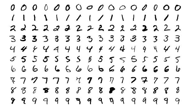
Figure 1: An example of digits from the MNIST dataset (Steppan, J., 2017).
Applications of machine learning
Non-medical applications of the machine include the following:
- Computer vision: camera calibration, activity recognition, character recognition, face recognition
- Natural language processing
- Speech recognition
- Recommender systems: Google, Netflix, Amazon
- Basic science: mathematics, biology, chemistry, physics
- Applied science: health care, self-driving cars
- Games: machine learning and artificial intelligence (AI) can compete in computer games. There are many examples of games such as GO, chess, and other computer related games. The award-winning documentary AlhpaGo demonstrates this, and the movie is available to stream on YouTube.
Medically-related applications include:
- Medical image processing: Medical image analysis incorporates the application of different imaging datasets of the human body for diagnosis or prognosis purposes. Commonly used imaging modalities are: Computed Tomography (CT), Magnetic Resonance Imaging (MRI), Positron Emission Tomography (PET), or even pathology images. The applications of medical image processing lead to diagnosed pathologies, survival prediction, guide medical interventions such as surgical planning, or for research purposes. Features extracted from medical images are called radiomics.
- Genetics: Genetics is the scientific study of genes and heredity. Due to the large size of gene sequences, machine learning helps to detect patterns connected to specific diseases. This act of mapping genes is known as genomics.
- Proteomics
- Radiogenomics: Combining radiomics (extracting data from medical images) with genetic information leads to finding imaging characteristics with their corresponding phenotypes.
- Multiomics: Multiomics provide a comprehensive understanding of molecular variations contributing to cellular response, diagnosis, and prognosis of diseases. This method uses an integration of omics for connecting diverse phenotypes as biomarkers.
Course objectives
This course aims to allow students to develop a machine learning (ML) toolbox that includes
- Formulating a problem as an ML problem
- Understanding a variety of ML algorithms
- Running and interpreting ML experiments
- Understanding what makes ML work – theory and practice
Python ![]()
Why was Python chosen for this course?
- A concise and intuitive language
- Simple, easy-to-learn syntax
- Highly readable, compact code
- Supports object-oriented and functional programming
- Strong support for integration with other languages (C, C++, Java)
- Cross-platform compatibility
- Many advanced models in machine learning are implemented with Python.
- Free
- Makes programming fun!
We assume you already know the basics of Python. That said, most of us can benefit from a little review, so we will do a quick guided walkthrough of some Python basics in the following notebook. You may also want to take advantage of A Whirlwind Tour of the Python Language.
Why Python for machine learning?
In the earliest days of computer science, it was a competition between the first high-level programming languages, namely Fortran and Lisp . This history is important because it highlights that the needs of AI programmers have historically differed significantly from other areas of computer science and Lisp accommodated these differences.
In recent years Python has emerged as the language of choice for machine learning and data science. Indeed, for those not fond of many nested parentheses, Python will be an improvement. Here are a few of the aspects of Python that make it a great choice for the needs of machine learning and data science:
- An interpreted language – allows for interactive data analysis
- Libraries for plotting and vector/matrix computation
- Many machine learning packages available: scikit-learn, TensorFlow, PyTorch
Language of choice for many machine learning practitioners, but some use/prefer R.
Python Anaconda ![]()
Use version 3.X of Python or more updated versions.
If setting up Python on your personal machine, we recommend the Anaconda Python distribution which is a data-science-oriented distribution that includes all the tools we will use in this course. Note that the smaller lighter Miniconda may serve you just fine.
IPython and the Jupyter Notebook
The Jupyter notebook is a browser-based interface to the IPython Python shell. In addition to executing Python/IPython statements, the notebook allows the user to include formatted text, static and dynamic visualizations, mathematical equations, and much more. It is the standard way of sharing data science analyses.
This course will be implemented in multiple Python Jupyter notebooks showing the ways to play with the data towards training a model and coming up with the final prediction.
Google Colab![]()
Please also consider setting yourself up to use Google Colab., You can pull the notebooks for the class directly from the github repository for the course by clicking the "open in colab" badge. If using Colab, make sure to copy the notebook to your google drive so that any changes you make will be saved. Jupyter notebook and Google Colab are entirely compatible with each other, and have a very similar interface.In course, we will briefly work with a deep neural network, which requires a using a graphcis processing unit (GPU), and Google Colab provides such an environment for this type ofprogramming.
Data preprocessing
The first and the most critical step in machine learning and data mining is data preprocessing. Most of the time data scientists spend more than 70% of their time to understand the data and prepare it for their analysis. In medical data analysis, data preprocessing is even more crucial due to its connection to patients’ health and its sensitivity.
What Is Data Preprocessing?
Data preprocessing is considered the most essential phase in the data analysis process. In this step, we take raw data and transform it into an understandable format, allowing computer machine learning models to access and easily analyze them.
Real-world medical data vary from different imaging modalities to patient clinical information and demographics. They are often messy and may contain inconsistencies, be incomplete, with an irregular or non-uniform design. A good machine learning design is directly related to how much the targeted data is nice and tidy. So structured data with numbers and percentages is easier to work with than unstructured data , which might be in the form of text or images and must first be cleaned and reformatted to quantitative values before analysis.
Data Preprocessing Importance
Many data scientists stress the idea of “garbage in, garbage out” when training machine learning models is. This means that having badly organized or dirty data lead to bad or undesirable outcomes. Another way to look at this is that sometimes we need to extract characteristics as much as possible, so as not to miss information, and that data need to be rearranged and organized before feeding it to the machine learning models. Data preprocessing is often more vital than applying the most powerful algorithms, and skippingthis important step may skew the analysis, resulting in a “garbage” output.
Depending on the data gathering methods and resources that we use, we may encounter data with out of range or incorrect features or meaningless values, e.g., negative value for cell count. One of the most common problem with data is having missing values or text data that need to be quantified. Properly preprocessed and cleaned data sets the system up for much more precise downstream processes. This is also directly connected to more accurate data-driven decision making. To the contrary, if the bad data drive the machine learning, bad decisions from the models will be inevitable.
Understanding Machine Learning Data Features
Features decode the information related to a targeted study into quantitative data that can be used for machine learning models. Such quantities can be location, size, age, time, temperature, blood pressure, etc. These attributes appear as columns of a dataset/spreadsheet, describing information about a specific individual measurable property or presenting a characteristic of an observed phenomenon.
Itis crucial to understand what the features describe before preprocessing them since deciding which ones to focus on relates directly to the applications’ goals Improving the quality the selected features allows for better processing and ultimately better decision making.
Similar to different types of measurements, qualitative and quantitative two types of features exist: categorical and numerical features.
- Categorical features:such features describe a category like different colors, diseases, types of animals, months of a year. Also they can be something that fits into one of two categories i.e., yes/no, true/false, right/left, positive/negative, etc. These features are considered to be predetermined in our analysis.
- Numerical features:these features involve a continuous or discrete measure i.e., statistical, scale or integer-related measures. Continuous numerical values can be weight, height, temperature, white blood cells count, time to an event, etc, which exhibit as an integer, floats (fraction), or percentages.
Sometimes the type of features that are used to train machine learning is higher level than quantitative measures i.e., text data or natural language processing data that need to be preprocessed and converted to quantitative attributes to be ready for a model.
Data Wrangling
Steps required for successfully preprocessing the data and making it ready for models must include the following:
- Data quality
Before doing anything, we need to have an idea about the overall quality of the data and its relevancy and consistency to objectives of the project. There are characteristic difficulties or anomalies that might exist with any data that need to be looked at:
- Data Types: Often we obtain data from various sources, which leads to different formatting. The ultimate goal for processing data is to make it readable for the machines, thus harmonization of datasets is needed. For instance, converting different dating systems, currencies, measure systems, etc.
- Data values: the purpose of this is to convert different descriptors of features so that they are uniformly explained.
- Outliers: Outliers can greatly affect data processing due to their extreme values. Outliers need to be removed from the analysis to mitigate the impact of them to the data.
- Discreditization: using more meaningful intervals provides much better information than specific factors. i.e., time difference or time average instead of specific time spent.
Implementation in Python
Data Type
The most straightforward way to implement data type conversion is by encoding the data. For example, converting names of specific places, locations, people, etc in the data to a machine-readable value. By encoding categorical data, they convert to integer values or categorical values that can be fed to a machine learning model and improve the predictions. Label encoding is probably the most basic type of categorical feature encoding techniques, which assigns a unique number to each categorical attribute. There is a method/function in the SKlearn Python library to execute encoding:
How to install scikitlearn library:
$ pip install -U scikit-learn
Import the sklearn library and use it for encoding the data:
$ from sklearn import preprocessing
$ encoder = preprocessing.LabelEncoder()
Data Value
To rescale data using sklearn.preprocessing method, we have:
$ X = np.array([[ 2.1, -11.2, 32.9],
[ 2.1, -11.2, 32.9],
[ 10.23, 31.8, -19.09]])
$ Rescal = preprocessing.StandardScaler()
$ Rescal = Rescal.fit(X)
$ scaledX = Rescal.transform(X)
$ scaledX
>>> array([[-0.69669583, -0.99995452, 1.3163266 ],
[-0.71746689, -0.36608753, -0.21043211],
[ 1.41416272, 1.36604205, -1.10589449]])
Normalization of an input is the process of scaling individual inputs to have unit norm. To normalize an input using sklearn we can use
$ X = [[ 1.2, -11.3, 24.3],
[ 32.7, 0.7, 0.98],
[ 10.78, 11.89, -91.9]]
$ X_norm = preprocessing.normalize(X, norm='l2')
$ X_norm
>>> array([[ 0.04473317, -0.42123731, 0.90584661],
[ 0.99932248, 0.02139222, 0.02994911],
[ 0.11555255, 0.12745081, -0.98509081]])
Missing information
There are several ways to deal with missing information such as replacing them with mean, median, zero, k-nearest neighbor (knn), and deep learning models. This process is called imputation. Sklearn has a method called SimpleImputer which can replace the missing data or NaN (Not a Number) with “mean”, “median”, and “most frequent” values.
$ from sklearn.impute import SimpleImputer
$ X = [[ 1.2, np.nan, 24.3],
[ 32.7, 0.7, 0.98],
[ 10.78, 11.89, np.nan]]
$ imp_mean = SimpleImputer( strategy='most_frequent')
$ imp_mean.fit(X)
$ imputed_x = imp_mean.transform(X)
$ imputed_x
>>> array([[ 1.2 , 6.295, 24.3 ],
[32.7 , 0.7 , 0.98 ],
[10.78 , 11.89 , 12.64 ]])
