
Chapter 4
Unsupervised Learning
Clustering methods
Unsupervised learning
Unsupervised learning is a type of machine learning where the algorithm is not given any labeled data to learn from. Instead, it is given a dataset of inputs and must find patterns or relationships in the data on its own. In unsupervised learning, the goal is to discover hidden structure in the data, such as clusters or lower-dimensional representations, rather than to make predictions or classify data points based on pre-existing labels. This can be useful for tasks such as data compression, anomaly detection, and data visualization.
Some common unsupervised learning algorithms include k-means clustering, hierarchical clustering, and dimensionality reduction techniques such as principal component analysis (PCA). These algorithms work by searching for patterns in the data and grouping similar data points together. They can also help in removing noise or reducing the dimensionality of the data. PCA is going to be discussed in its our chapter, but clustering methods are briefly explained here. unsupervised learning is a type of machine learning where the algorithm is not given labeled data and must find relationships in the data on its own, in order to uncover hidden structure or patterns.
The k–means clustering algorithm
In the clustering problem, we are given a training set [latex]\{x^{(1)},…,x^{(m)}\}[/latex], and want to group the data into a few cohesive clusters. Here, [latex]x^{(i)}∈\mathbb{R}^n[/latex] as usual; but no labels [latex]y^{(i)}[/latex] are given. So, this is an unsupervised learning problem.
The k-means clustering algorithm is as follows:
- 1.Initialize cluster centroids [latex]\mu_1,\mu_2,…,\mu_k∈\mathbb{R}^n[/latex] randomly.
- 2.Repeat until convergence: {
- For every [latex]i[/latex], set
[latex]c^{(i)} := \underset{j}{argmin}||x^{(i)} - \mu_j||^2[/latex]
-
- For each j, set
[latex]\mu_j := \frac{\sum_{i = 1}^m 1 \{c^{(i)} = j\} x^{(i)}}{\sum_{i=1}^m 1\{c^{(i)}=j\}}.[/latex]
-
- }
In the algorithm above, k (a parameter of the algorithm) is the number of clusters we want to find; and the cluster centroids [latex]\mu_j[/latex]represent our current guesses for the positions of the centers of the clusters. To initialize the cluster centroids (in step 1 of the algorithm above), we could choose k training examples randomly, and set the cluster centroids to be equal to the values of these k examples. (Other initialization methods are also
possible.)
The inner-loop of the algorithm repeatedly carries out two steps: (i) Assigning each training example [latex]x^{(i)}[/latex] to the closest cluster centroid [latex]\mu_{j}[/latex], and (ii) Moving each cluster centroid [latex]\mu_j[/latex] to the mean of the points
assigned to it. Figure 4.1 shows an illustration of running k-means.
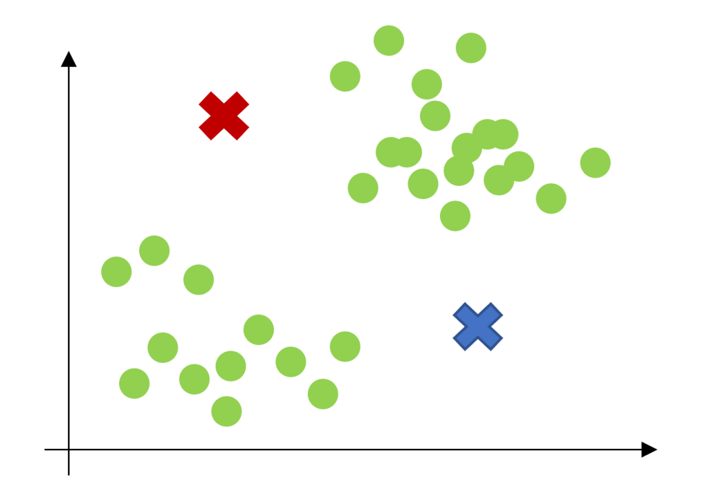
Figure 4.1
Is the k-means algorithm guaranteed to converge? Yes it is, in a certain sense. In particular, let us define the distortion function to be:
[latex]J(c,\mu) = \sum_{i=1}^m||x^{(i)}-\mu_{c^{(i)}}||^2\tag{4.1}[/latex]
Thus, J measures the sum of squared distances between each training example [latex]x^{(i)}[/latex] and the cluster centroid [latex]\mu_{c^{(i)}}[/latex] to which it has been assigned. It can be shown that k-means is exactly coordinate descent on J. Specifically, the inner-loop of k-means repeatedly minimizes J with respect to c while holding µ fixed, and then minimizes J with respect to µ while holding c fixed. Thus, J must monotonically decrease, and the value of J must converge. (Usually, this implies that c and µ will converge too. In theory, it is possible for k-means to oscillate between a few different clustering i.e., a few different values for c and/or µ that have exactly the same value of J, but this almost never happens in practice.)
The distortion function J is a non-convex function, and so coordinate descent on J is not guaranteed to converge to the global minimum. In other words, k-means can be susceptible to local optima. Very often k-means will work fine and come up with very good clustering despite this. But if you are worried about getting stuck in bad local minima, one common thing to do is run k-means many times (using different random initial values for the cluster centroids [latex]\mu_j[/latex]). Then, out of all the different clusterings found, pick the one that gives the lowest distortion [latex]J(c;\mu).[/latex]
Mixtures of Gaussians and the EM algorithm
In this set of notes, we discuss the EM (Expectation-Maximization) for density estimation. Suppose that we are given a training set [latex]\{x^{(1)},…,x^{(m)}\}[/latex], as usual. Since we are in the unsupervised learning setting, these points do not come with any labels.
We wish to model the data by specifying a joint distribution [latex]p(x^{(i)},y^{(i)})=p(x^{(i)}|z^{(i)})p(z^{(i)})[/latex]. Here, [latex]z^{(i)}[/latex] Multinomial([latex]\Phi[/latex]) (where [latex]\Phi_j ≥ 0, \sum_{j=1}^k \Phi_j =1[/latex], and the parameter [latex]\Phi_j[/latex] gives [latex]p(z^{(i)}=j)[/latex].), and [latex]x^{(i)}|z^{(i)}= j∼N(\mu_j; Σ_j).[/latex] We let k denote the number of values that the [latex]z^{(i)}[/latex]‘s can take on. Thus, our model posits that each [latex]x^{(i)}[/latex] was generated by randomly choosing [latex]z^{(i)}[/latex] from [latex]\{1,…,k\}[/latex], and then [latex]x^{(i)}[/latex] was drawn from one of k Gaussians depending on [latex]z^{(i)}[/latex].
This is called the mixture of Gaussians model. Also, note that the [latex]z^{(i)}[/latex]‘s are latent random variables, meaning that they’re hidden/unobserved. This is what will make our estimation problem difficult. The parameters of our model are thus [latex]\Phi,\mu[/latex] and [latex]Σ[/latex]. To estimate them, we can write down the likelihood of our data:
[latex]\begin{align*} \ell ( \Phi, \mu, Σ) &= \sum_{i=1}^m \text{log } \ p (x^{(i)}; \Phi, \mu, Σ) \\ &= \sum_{i=1}^m \text{log } \sum_{z^{(i)}=1}^k p(x^{(i)}|z^{(i)} ; \mu, Σ) p(z^{(i)};\Phi).\tag{4.2} \end{align*}[/latex]
However, if we set to zero the derivatives of this formula with respect to the parameters and try to solve, we’ll find that it is not possible to find the maximum likelihood estimates of the parameters in closed form. (Try this yourself at home.) The random variables [latex]z^{(i)}[/latex] indicate which of the k Gaussians each [latex]x^{(i)}[/latex] had come from. Note that if we knew what the [latex]z^{(i)}[/latex]‘s were, the maximum likelihood problem would have been easy. Specifically, we could then write down the likelihood as
[latex]\ell (\Phi, \mu, Σ) = \sum_{i=1}^k \text{log } \ p(x^{(i)}|z^{(i)} ; \mu, Σ) + \text{log } \ p(z^{(i)} ; \Phi).\tag{4.3}[/latex]
Maximizing this with respect to [latex]\Phi,\mu[/latex] and [latex]Σ[/latex] gives the parameters:
[latex]\begin{align*} \Phi_j &= \frac{1}{m}\sum_{i=1}^m 1\{ z^{(i)} = j \},\\ \mu_j &= \frac{\sum_{i=1}^m 1\{z^{(i)} = j\}x^{(i)}}{\sum_{i=1}^m 1\{ z^{(i)}=j\}}, \\ Σ_j &= \frac{\sum_{i=1}^m 1\{z^{(i)} = j \} (x^{(i)} - \mu_j)(x^{(i)}-u_j)^T}{\sum_{i=1}^m 1\{ z^{(i)} = j \}}.\tag{4.4}\end{align*}[/latex]
Indeed, we see that if the [latex]z^{(i)}[/latex]‘s were known, then maximum likelihood estimation becomes nearly identical to what we had when estimating the parameters of the Gaussian discriminant analysis model, except that here the [latex]z^{(i)}[/latex]‘s playing the role of the class labels.
However, in our density estimation problem, the [latex]z^{(i)}[/latex]‘s are not known. What can we do? The EM algorithm is an iterative algorithm that has two main steps. Applied to our problem, in the E-step, it tries to guess the values of the [latex]z^{(i)}[/latex]‘s. In the M-step, it updates the parameters of our model based on our guesses. Since in the M-step we are pretending that the guesses in the first part were correct, the maximization becomes easy. Here’s the algorithm:
- Repeat until convergence: {
- (E-step) For each i; j, set
[latex]w_j^{(i)} := p (z^{(i)} = j | x^{(i)} ; \Phi, \mu, Σ)[/latex]
-
- (M-step) Update the parameters:
\begin{align*} \Phi_j & := \frac{1}{m}\sum_{i=1}^mw_j^{(i)},\\ \mu_j &:= \frac{\sum_{i=1}^m w_j^{(i)}x^{(i)}}{\sum_{i=1}^mw_j^{(i)}}, \\ Σ_j &:= \frac{Σ_{i=1}^mw_j^{(i)}(x^{(i)}-\mu_j)(x^{(i)}-\mu_j)^T}{\sum_{i=1}^mw_j^{(i)}}
\end{align*}
- }
In the E-step, we calculate the posterior probability of our parameters the [latex]z^{(i)}[/latex]‘s, given the [latex]x^{(i)}[/latex] and using the current setting of our parameters. I.e., using Bayes rule, we obtain:
[latex]P(z^{(i)} = j|x^{(i)} ; \Phi, \mu, Σ) = \frac{p(x^{(i)}|z^{(i)} = j;\mu, Σ) \ p (z^{(i)} = j; \Phi)}{\sum_{l=1}^k p (x^{(i)}|z^{(i)}=l;\mu,Σ) \ p(z^{(i)}= l; \Phi)}\tag{4.5}[/latex]
Here, [latex]p ( x^{(i)}|z^{(i)} = j;\mu,Σ)[/latex] is given by evaluating the density of a Gaussian with mean [latex]\mu_j[/latex] and covariance [latex]Σ_j[/latex] at [latex]x^{(i)}; p(z^{(i)}=j,Φ)[/latex] is given by [latex]\phi_j[/latex], and so on. The values [latex]w_j^i[/latex] calculated in the E-step represent our soft guesses for the values of [latex]z^{(i)}[/latex].
Also, you should contrast the updates in the M-step with the formulas we had when the [latex]z^{(i)}[/latex]‘s were known exactly. They are identical, except that instead of the indicator functions ”[latex]1\{z^{(i)}=j\}[/latex]” indicating from which Gaussian each datapoint had come, we now instead have the [latex]w_j^{(i)}[/latex]‘s.
The EM-algorithm is also reminiscent of the K-means clustering algorithm, except that instead of the hard cluster assignments [latex]c(i)[/latex], we instead have the soft assignments [latex]w_j^i[/latex]. Similar to K-means, it is also susceptible to local optima, so reinitializing at several different initial parameters may be a good idea.
It’s clear that the EM algorithm has a very natural interpretation of repeatedly trying to guess the unknown [latex]z^{(i)}[/latex]‘s; but how did it come about, and can we make any guarantees about it, such as regarding its convergence? In the next set of notes, we will describe a more general view of EM, one that will allow us to easily apply it to other estimation problems in which there are also latent variables, and which will allow us to give a convergence guarantee.
The EM algorithm
In the previous set of notes, we talked about the EM algorithm as applied to fitting a mixture of Gaussians. In this set of notes, we give a broader view of the EM algorithm, and show how it can be applied to a large family of estimation problems with latent variables. We begin our discussion with a very useful result called Jensen’s inequality.
Jensen’s inequality
Let f be a function whose domain is the set of real numbers. Recall that f is a convex function if [latex]f''(x)≥0[/latex] (for all [latex]x∈\mathbb{R}[/latex]). In the case of f taking vector-valued inputs, this is generalized to the condition that its hessian H is positive semi-definite ( [latex]H≥0[/latex]). If [latex]f''(x)>0[/latex] for all x, then we say f is strictly convex (in the vector-valued case, the corresponding statement is that H must be positive [latex]definite[/latex], written H>0). Jensen’s inequality can then be stated as follows:
Theorem. Let f be a convex function, and let X be a random variable. Then:
[latex]E[f(x)]≥f[EX].\tag{4.6}[/latex]
Moreover, if f is strictly convex, then [latex]E[f(X)]=f(EX)[/latex] holds true if and only if [latex]X=E[X][/latex] with probability 1 (i.e., if X is a constant).
Recall our convention of occasionally dropping the parentheses when writing expectations, so in them theorem above, [latex]f(EX)=f(E[X])[/latex]. For an interpretation of the theorem, consider the figure below.
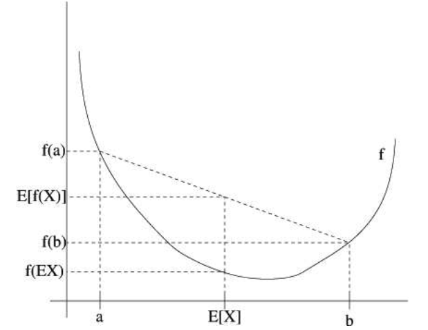
Figure 4.2
Here, f is a convex function shown by the solid line. Also, X is a random variable that has a 0.5 chance of taking the value a, and a 0.5 chance of taking the value b (indicated on the x-axis). Thus, the expected value of X is given by the midpoint between a and b.
We also see the values f (a), f (b) and [latex]f(E[X])[/latex] indicated on the y-axis. Moreover, the value [latex]E[f(X)][/latex] is now the midpoint on the y-axis between f (a) and f (b). From our example, we see that because f is convex, it must be the case that [latex]E[f(X)]≥f(EX)[/latex].
Incidentally, quite a lot of people have trouble remembering which way the inequality goes, and remembering a picture like this is a good way to quickly figure out the answer.
Remark. Recall that f is [strictly] concave if and only if –f is [strictly] convex (i.e., [latex]f''(x)≤0[/latex] or [latex]H≤0[/latex]). Jensen’s inequality also holds for concave functions f, but with the direction of all the inequalities reversed ( [latex]E[f(X)]≤f(EX)[/latex], etc.).
The EM algorithm
Suppose we have an estimation problem in which we have a training set [latex]\{x^{(1)},…,x^{(m)}\}[/latex] consisting of m independent examples. We wish to fit the parameters of a model [latex]p(x,z)[/latex] to the data, where the likelihood is given by
[latex]\ell (θ)=\sum_{i=1}^m\text{log } \ p(x,θ)=\sum_{i=1}^m \text{log } ∑_zp(x,z;θ).\tag{4.7}[/latex]
But, explicitly finding the maximum likelihood estimates of the parameters θ may be hard. Here, the [latex]z^{(i)}[/latex]‘s are the latent random variables; and it is often the case that if the [latex]z^{(i)}[/latex]‘s were observed, then maximum likelihood estimation would be easy.
In such a setting, the EM algorithm gives an efficient method for maximum likelihood estimation. Maximizing [latex]\ell (θ)[/latex] explicitly might be di‑cult, and our strategy will be to instead repeatedly construct a lowerbound on [latex]\ell[/latex](E-step), and then optimize that lower-bound (M-step). For each i, let [latex]Q_i[/latex] be some distribution over the z‘s [latex](∑_zQ_i(z)=1,Q_i(z)≥0[/latex]). Consider the following:
[latex]\begin{align*} \sum_i \text{log } \ p(x^{(i)}; θ) &= \sum_i \text{log } \sum_{z^{(i)}} p (x^{(i)},z^{(i)}; θ) \tag{4.8}\\ &= \sum_i \text{log } \sum_{z^{(i)}} Q_{i}(z^{(i)}) \frac{p(x^{(i)},z^{(i)}; θ)}{Q_i(z^{(i)})} \tag{4.9}\\ & \geq \sum_i \sum_{z^{(i)}}Q_i(z^{(i)})\text{log }\frac{p(x^{(i)},z^{(i)};θ)}{Q_i(z^{(i)})} \tag{4.10} \end{align*}[/latex]
The last step of this derivation used Jensen’s inequality. Specifically, [latex]f(x)=\text{log } x[/latex] is a concave function, since [latex]f''(x)=-1/x^{2}<0[/latex] over its domain [latex]x ∈\mathbb{R}^+.[/latex] Also, the term
[latex]\sum_{z^{(i)}} Q_i (z^{(i)}) \left[\frac{p(x^{(i)},z^{(i)};θ)}{Q_i (z^{(i)})}\right]\tag{4.11}[/latex]
in the summation is just an expectation of the quantity [latex][p(x^{(i)},z^{(i)};θ)/Q_i(z^{(i)})][/latex] with respect to [latex]z^{(i)}[/latex] drawn according to the distribution given by [latex]Q_i[/latex]. By Jensen’s inequality, we have
[latex]f \left( E_{z^{(i)}\sim Q_i} \left[\frac{p(x^{(i)},z^{(i)};θ)}{Q_i (z^{(i)})}\right] \right) \geq E_{z^{(i)}\sim Q_i}\left[f \left(\frac{p(x^{(i)},z^{(i)};θ)}{Q_i (z^{(i)})}\right)\right]. \tag{4.12}[/latex]
where the [latex]z^{(i)}\sim Q_i[/latex] subscripts above indicate that the expectations are with respect to [latex]z^{(i)}[/latex] drawn from [latex]Q_i[/latex]. This allowed us to go from (4.8) to (4.10).
Now, for any set of distributions [latex]Q_i[/latex], the formula (4.10) gives a lower-bound on [latex]\ell (θ)[/latex]. There’re many possible choices for the [latex]Q_i[/latex]‘s. Which should we choose? Well, if we have some current guess θ of the parameters, it seems natural to try to make the lower-bound tight at that value of θ. I.e., we’ll make the inequality above hold with equality at our particular value of θ. (We’ll see later how this enables us to prove that [latex]\ell (θ)[/latex] increases monotonically with successive iterations of EM.) To make the bound tight for a particular value of θ, we need for the step involving Jensen’s inequality in our derivation above to hold with equality. For this to be true, we know it is su‑cient that that the expectation be taken over a constant-valued random variable. I.e., we require that
[latex]\frac{p(x^{(i)},z^{(i)}; θ)}{Q_i(z^{(i)})} = c\tag{4.13}[/latex]
for some constant c that does not depend on [latex]z^{(i)}[/latex]. This is easily accomplished by choosing
[latex]Q_i(z^{(i)}) \propto p (x^{(i)}, z^{(i)};θ).\tag{4.14}[/latex]
Actually, since we know [latex]∑_zQ_i(z^{(i)})=1[/latex] (because it is a distribution), this further tells us that
[latex]\begin{align*} Q_i(z^{(i)}) &= \frac{p(x^{(i)},z^{(i)};θ)}{\sum_z p(x^{(i)}, z;θ)}\\ &= \frac{p(x^{(i)},z^{(i)};θ)}{p(x^{(i)};θ) }\\ &= p(z^{(i)} | x^{(i)} ; θ) \tag{4.15}\end{align*}[/latex]
Thus, we simply set the [latex]Q_i[/latex]‘s to be the posterior distribution of the [latex]z^{(i)}[/latex]‘s given [latex]x^{(i)}[/latex] and the setting of the parameters θ.
Now, for this choice of the [latex]Q_i[/latex]‘s, Equation (4.10) gives a lower-bound on the loglikelihood ‘ that we’re trying to maximize. This is the E-step. In the M-step of the algorithm, we then maximize our formula in Equation (4.10) with respect to the parameters to obtain a new setting of the θ‘s. Repeatedly carrying out these two steps gives us the EM algorithm, which is as follows:
- Repeat until convergence {
- (E-step) For each i, set
[latex]Q_i(z^{(i)}) := p ( z^{(i)} | x^{(i)} ; θ)[/latex]
-
- (M-step) Set
[latex]θ := \underset{θ}{argmax} \sum_i \sum_{z^{(i)}}Q_i\left(z^{(i)} \right)\text{log } \frac{p(x^{(i)},z^{(i)}; θ)}{Q_i(z^{(i)})}[/latex]
- }
How will we know if this algorithm will converge? Well, suppose [latex]θ^{(t)}[/latex] and [latex]θ^{(t+1)}[/latex] are the parameters from two successive iterations of EM. We will now prove that [latex]\ell(θ^{(t)}) ≤ \ell (θ^{(t+1)})[/latex], which shows EM always monotonically improves the log-likelihood. The key to showing this result lies in our choice of the [latex]Q_i[/latex]‘s. Specifically, on the iteration of EM in which the parameters had started out as [latex]θ^{(t)}[/latex], we would have chosen [latex]Q_i^{(t)}z^{(i)}:=p(z^{(i)}|x^{(i)};θ^{(t)})[/latex]. We saw earlier that this choice ensures that Jensen’s inequality, as applied to get (4.10), holds with equality, and hence
[latex]\ell\left(θ^{(t)}\right) = \sum_i\sum_{z^{(i)}}Q_i^{(t)}\left(z^{(i)}\right) \text{log } \frac{p (x^{(i)}, z^{(i)};θ^{(t)})}{Q_i^{(t)} \left( z^{(i)}\right)}.\tag{4.16}[/latex]
The parameters [latex]θ^{(t+1)}[/latex] are then obtained by maximizing the right hand side of the equation above. Thus,
\begin{align*}\ell(θ^{(t+1)}) & \geq \sum_i \sum_{x^{(i)}}Q_i^{(t)} (z^{(i)}) \text{log } \frac{p(x^{(i)},z^{(i)} ; θ^{(t+1)})}{Q_i^{(t)}(z^{(i)})}\tag{4.17} \\ & \geq \sum_i \sum_{z^{(i)}} Q_i^{(t)} (z^{(i)}) \text{log } \frac{p(x^{(i)}, z^{(i)}; θ^{(t)})}{Q_i^{(t)}(z^{(i)})}\tag{4.18} \\ & =\ell(θ^{(t)})\tag{4.19} \end{align*}
This first inequality comes from the fact that
[latex]\ell(θ) \geq \sum_i \sum_{z^{(i)}}Q_i\left(z^{(i)}\right) \text{log } \frac{p(x^{(i)},z^{(i)};θ)}{Q_i(z^{(i)})}\tag{4.20}[/latex]
holds for any values of [latex]Q_i[/latex] and θ, and in particular holds for [latex]Q_i=Q_i^{(t)},θ=θ^{(t+1)}[/latex]. To get Equation (4.17), we used the fact that [latex]θ^{(t+1)}[/latex] is chosen explicitly to be
[latex]\underset{θ}{argmax}\sum_i\sum_{z^{(i)}} Q_i\left(z^{(i)}\right) \text{log } \frac{p(x^{(i)},z^{(i)};θ)}{Q_i(z^{(i)})}\tag{4.21}[/latex]
and thus this formula evaluated at [latex]θ^{(t+1)}[/latex] must be equal to or larger than the same formula evaluated at [latex]θ^{(t)}[/latex]. Finally, the step used to get (4.19) was shown earlier, and follows from [latex]Q_i^t[/latex] having been chosen to make Jensen’s inequality hold with equality at [latex]θ^{(t)}[/latex].
Hence, EM causes the likelihood to converge monotonically. In our description of the EM algorithm, we said we’d run it until convergence. Given the result that we just showed, one reasonable convergence test would be to check if the increase in [latex]\ell (θ)[/latex] between successive iterations is smaller than some tolerance parameter, and to declare convergence if EM is improving [latex]\ell (θ)[/latex] too slowly.
Remark. If we define
[latex]J(Q,θ) = \sum_i \sum_{z^{(i)}}Q_i \left(z^{(i)}\right) \text{log } \frac{p(x^{(i)},z^{(i)};θ)}{Q_i(z^{(i)})},\tag{4.22}[/latex]
then we know [latex]\ell (θ)≥J(Q;θ)[/latex] from our previous derivation. The EM can also be viewed a coordinate ascent on J, in which the E-step maximizes it with respect to Q (check this yourself), and the M-step maximizes it with respect to θ.
Mixture of Gaussians revisited
Armed with our general definition of the EM algorithm, let’s go back to our old example of fitting the parameters Φ, µ and Σ in a mixture of Gaussians. For the sake of brevity, we carry out the derivations for the M-step updates only for Φ and [latex]\mu_j[/latex], and leave the updates for [latex]Σ_j[/latex] as an exercise for the reader. The E-step is easy. Following our algorithm derivation above, we simply calculate
[latex]w_j^{(i)} = Q_i \left(z^{(i)} = j \right) = P \left(z^{(i)} = j|x^{(i)}; Φ, \mu, Σ \right).\tag{4.23}[/latex]
Here, “[latex]Q_i(z^{(i)}=j)[/latex]” denotes the probability of [latex]z^{(i)}[/latex] taking the value j under the distribution [latex]Q_{i}[/latex].
Next, in the M-step, we need to maximize, with respect to our parameters [latex]Φ;\mu;Σ[/latex], the quantity
[latex]\sum_{i=1}^m\sum_{z^{(i)}}Q_i (z^{(i)}) \text{ log } \frac{p(x^{(i)},z^{(i)};Φ,\mu,Σ)}{Q_i(z^{(i)})}[/latex]
[latex]= \sum_{i=1}^m \sum_{j=1}^k Q_i(z^{(i)} = j) \text{ log }\frac{p(x^{(i)}|z^{(i)}=j;\mu,Σ)p(z^{(i)}=j;Φ)}{Q_i(z^{(i)}=j)}[/latex]
[latex]= \sum_{i=1}^m \sum_{j=1}^k w_j^{(i)} \text{ log }\frac{\frac{1}{(2\pi)^{n/2}|Σ_j|^{1/2}}exp\left(-\frac{1}{2}(x^{(i)}-\mu_j)^TΣ_j^{-1}(x^{(i)}-\mu_j)\right)\cdot Φ_j}{w_j^{(i)}}\tag{4.24}[/latex]
Let’s maximize this with respect to [latex]\mu_l[/latex]. If we take the derivative with respect to [latex]\mu_l[/latex], we find
\begin{array}{rc} & ∇_{\mu_l} \sum_{i=1}^m \sum_{j=1}^k w_j^{(i)} \text{ log }\frac{\frac{1}{(2\pi)^{n/2}|Σ_j|^{1/2}}exp\left(-\frac{1}{2}(x^{(i)}-\mu_j)^TΣ_j^{-1}(x^{(i)}-\mu_j)\right)\cdot Φ_j}{w_j^{(i)}}\\ = & -∇_{\mu_l} \sum_{i=1}^m \sum_{j=1}^k w_j^{(i)} \frac{1}{2}(x^{(i)}-\mu_j)^T Σ_j^{-1}\left(x^{(i)} – \mu_j \right)\\ =&\frac{1}{2}\sum_{i=1}^m w_l^{(i)}∇_{\mu_l}2\mu_l^T Σ_l^{-1} x^{(i)} – \mu_l^T Σ_l^{-1} \mu_l \\ =& \sum_{i=1}^m w_l^{(i)}\left(Σ_l^{-1}x^{(i)}-Σ_j^{-1} \mu_l \right) \tag{4.25} \end{array}
Setting this to zero and solving for [latex]\mu_l[/latex] therefore yields the update rule
[latex]\mu_l := \frac{\sum_{i=1}^m w_l^{(i)}x^{(i)}}{\sum_{i=1}^mw_l^{(i)}},\tag{4.26}[/latex]
which was what we had in the previous set of notes.
Let’s do one more example, and derive the M-step update for the parameters [latex]Φ_j[/latex]. Grouping together only the terms that depend on [latex]Φ_j[/latex], we find that we need to maximize
[latex]\sum_{i=1}^m\sum_{j=1}^kw_j^{(i)}\text{ log }Φ_j.\tag{4.27}[/latex]
However, there is an additional constraint that the [latex]Φ_j[/latex]‘s sum to 1, since they represent the probabilities [latex]Φ_j=p(z^{(i)}=j;Φ)[/latex]. To deal with the constraint that [latex]\sum_{j=1}^kΦ_j=1[/latex], we construct the Lagrangian
[latex]\mathcal{L}(Φ) = \sum_{i=1}^m\sum_{j=1}^kw_j^{(i)}\text{ log }Φ_j + \beta\left(\sum_{j=1}^k Φ_j - 1\right)\tag{4.28}[/latex],
where β is the Lagrange multiplier Taking derivatives, we find We don’t need to worry about the constraint that [latex]Φ_j \geq 0[/latex], because as we’ll shortly see, the solution we’ll find from this derivation will automatically satisfy that anyway.
[latex]\frac{∂}{∂Φ_j}\mathcal{L}(Φ) = \sum_{i=1}^m \frac{w_j^{(i)}}{Φ_j}+1[/latex]
Setting this to zero and solving, we get
[latex]Φ_j= \frac{\sum_{i=1}^mw_j^{(i)}}{-\beta}\tag{4.29}[/latex]
i.e., [latex]Φ_j ∝ ∑_{i=1}^mw_j^{(i)}=1.[/latex] Using the constraint that [latex]∑_jΦ_j=1[/latex], we easily find that [latex]-\beta = \sum_{i = 1}^m \sum_{j=1}^k w_j^{(i)}=\sum_i^m 1 = m[/latex] (This used the fact that [latex]w_j^{(i)} = Q_i(z^{(i)}=j)[/latex], and since probabilities sum to 1, [latex]\sum_jw_j^{(i)} = 1.[/latex]) We therefore have our M-step updates for the parameters [latex]Φ_j[/latex]:
[latex]Φ_j := \frac{1}{m}\sum_{i=1}^mw_j^{(i)}.\tag{4.30}[/latex]
The derivation for the M-step updates to [latex]Σ_j[/latex] are also entirely straightforward.
Source: Machine Learning (Course). Andrew Ng. Openstax CNX (Rice University) 2013. https://cnx.org/contents/THQBCjjQ@4.2:AifRdKFz@2/Machine-Learning-Introduction
