Chapter 3

Classification Analysis

Supervised learning

Introduction to classification
Classification, a fundamental pillar of machine learning, empowers us to uncover patterns, classify data into distinct categories, and make predictions about future observations. In this chapter, we embark on a captivating journey into the realm of classification, exploring its principles, methodologies, and applications.

3.1 The Significance of Classification.

In a world abundant with data, understanding and organizing information into meaningful categories is of paramount importance. Classification provides a powerful framework for discerning patterns, distinguishing between different classes, and making informed decisions based on available evidence. Whether it’s detecting fraudulent transactions, identifying spam emails, or diagnosing diseases, classification algorithms serve as invaluable tools across diverse domains.

3.2 Fundamentals of Classification

To lay a solid foundation, we delve into the fundamental concepts of classification. We explore the notion of class labels and feature vectors, understanding their roles in the classification process. Additionally, we discuss the importance of labeled training data, which serves as the basis for building robust and accurate classification models.

3.3 Binary Classification

In this section, we delve into the realm of binary classification, where the task is to assign data instances to one of two possible classes. We explore popular algorithms such as logistic regression, support vector machines, and decision trees, uncovering their underlying principles and discussing their strengths and limitations. We also delve into techniques for evaluating the performance of binary classifiers, including precision, recall, and the receiver operating characteristic (ROC) curve.

3.4 Multiclass Classification

Building upon the foundations of binary classification, we extend our exploration to the realm of multiclass classification. Here, the objective is to assign instances to multiple classes. We examine powerful algorithms such as multinomial logistic regression, k-nearest neighbors, and ensemble methods like random forests and gradient boosting. We discuss strategies for handling imbalanced data, and techniques such as one-vs-rest and one-vs-one approaches.

3.5 Evaluating Classification Models

Assessing the performance of classification models is crucial to gauge their effectiveness and reliability. In this section, we delve into various evaluation metrics such as accuracy, precision, recall, F1-score, and area under the ROC curve. We discuss cross-validation techniques, model selection, and hyperparameter tuning to ensure the robustness and generalizability of classification models.

3.6 Handling Challenges in Classification

Real-world classification tasks often present unique challenges that require specialized approaches. We explore strategies for handling class imbalance, dealing with missing data, and addressing the curse of dimensionality. We also discuss techniques such as feature selection, dimensionality reduction, and ensemble learning to enhance the performance and interpretability of classification models.

3.7 Advanced Classification Techniques

In the final section of this chapter, we delve into advanced classification techniques that push the boundaries of traditional approaches. We explore the realm of deep learning, convolutional neural networks, recurrent neural networks, and transfer learning. These cutting-edge methods enable us to tackle complex classification problems, leverage unstructured data, and unlock new opportunities for accurate and insightful predictions.

As we embark on this journey into the world of classification, we equip ourselves with the tools to uncover patterns, classify data accurately, and make informed predictions. By understanding the principles, methodologies, and applications of classification in machine learning, we pave the way for solving real-world challenges and extracting actionable insights from complex data.

Classification and logistic regression
The classification problem in machine learning involves predicting discrete values, as opposed to the continuous values in the regression problem. One specific type of classification problem is binary classification, in which the predicted values can only be one of two options, such as 0 or 1. For example, in the task of building a spam classifier for email, the input data [latex](x^{(i)})[/latex] may include features of a particular email, and the output [latex](y)[/latex] would be 1 if the email is considered spam, and 0 if it is not. These two possible output values are commonly referred to as the “negative class” (0) and “positive class” (1), and can also be denoted using the symbols “-” and “+” respectively. The output value [latex](y^{(i)})[/latex] for a given input data point [latex](x^{(i)})[/latex] is also known as the label for that training example.

Logistic regression
The classification problem can be approached using the same linear regression algorithm as used for regression problems, but this approach may not yield optimal results. This is because a linear regression model would output continuous values for y, rather than the discrete values of 0 or 1 that are expected in a classification problem. Additionally, the predicted values for [latex]h_θ(x)[/latex] would not be restricted to the range of 0 to 1, which is not appropriate for a classification problem where y can only take on the values of 0 or 1. Therefore, it is important to consider the discrete nature of the output values in classification problems and use appropriate algorithms that can handle this constraint, [latex]y ∈ \{0,1\}[/latex]. To fix this, let’s change the form for our hypotheses [latex]h_θ(x)[/latex]. We will choose

[latex]h_θ(x)=g(θ^Tx)=\frac{1}{1+e^{-θ^Tx}}\tag{3.1},[/latex]

where

[latex]g(z)=\frac{1}{1+e^{-z}}\tag{3.2}[/latex]

is called the logistic function or the sigmoid function. Here is a plot showing [latex]g(z)[/latex]:

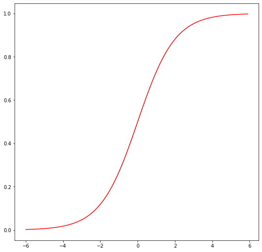
Figure 3.1

Notice that [latex]g(z)[/latex] tends towards 1 as [latex]z→∞[/latex], and [latex]g(z)[/latex] tends towards 0 as [latex]z→-∞[/latex]. Moreover, [latex]g(z)[/latex], and hence also [latex]h(x)[/latex], is always bounded between 0 and 1. As before, we are keeping the convention of letting [latex]x_0=1[/latex], so that [latex]θ^Tx=θ_0+\sum_{j = 1}^n θ_j x_j[/latex]
The logistic function, also known as the sigmoid function, is a common choice for the function [latex]g[/latex] in a classification problem. The logistic function smoothly increases from 0 to 1, making it a suitable function to model the probability that a given input belongs to the positive class. However, it is worth noting that other functions that exhibit this behavior can also be used. The choice of the logistic function becomes more natural when discussing Generalized Linear Models (GLMs) and generative learning algorithms. Additionally, the derivative of the sigmoid function, [latex]g'[/latex], has a useful property that can be utilized in the optimization process.

[latex]\begin{align*}g'(z) &= \frac{d}{dz}\frac{1}{1+e^{-z}}\\ &=\frac{1}{(1+e-z)^2}(e^{-z})\\ &=\frac{1}{1+e^{-z}}\cdot \left( 1-\frac{1}{1+e^{-z}}\right)\\ &= g(z)(1-g(z)). \tag{3.3}\end{align*}[/latex]

Once the logistic regression model is defined, the next step is to determine the optimal values for the parameters [latex]θ[/latex]. One way to do this is to use the method of maximum likelihood estimation. This method involves endowing the classification model with a set of probabilistic assumptions, and then using these assumptions to find the values of [latex]θ[/latex] that maximize the likelihood of the observed data. This approach is similar to how least squares regression can be derived as the maximum likelihood estimator under certain assumptions. Maximum likelihood estimation is a widely used method for fitting parameters in probabilistic models, and is particularly well-suited for logistic regression due to its probabilistic nature. Let us assume that

[latex]P(y=1|x;θ)=h_θ(x)[/latex]

[latex]P(y=0|x;θ)=1-h_θ(x)\tag{3.4}[/latex]

Note that this can be written more compactly as

[latex]p(y|x;θ)=(h_θ(x))^y(1-h_θ(x))^{1-y}\tag{3.5}[/latex]

When assuming that the m training examples were independently generated, the likelihood of the parameters can be expressed mathematically as the product of the probability of each individual training example given the corresponding input data and the current parameter values. This can be written as:

[latex]\begin{align*}L(θ)&=p(y⃗|X;θ)\\ &=\prod_{i=1}^mp(y^{(i)}|x^{(i)};θ)\\ &=\prod_{i=1}^m(h_θ(x^{(i)}))^{y^{(i)}}(1-hθ(x^{(i)}))^{1-y^{(i)}}\tag{3.6} \end{align*}[/latex]

As before, it will be easier to maximize the log likelihood:

[latex]\begin{align*} \ell(θ) &= \text{log }L(θ)\\ &= \sum_{i=1}^{m}y^{(i)}\text{log }h(x^{(i)})+(1-y^{(i)})\text{log }\left(1-h(x^{(i)})\right) \tag{3.7}\end{align*}[/latex]

One way to maximize the likelihood of the parameters is to use a method called gradient ascent. This method involves iteratively updating the parameter values in the direction of the gradient of the likelihood function with respect to the parameters. The updates for the parameters using gradient ascent can be written in vector notation as:

[latex]θ := θ + α ∇_θ \ell(θ) \tag{3.8}[/latex]

Where α is the learning rate and [latex]∇_θ\ell(θ)[/latex] represents the gradient of the likelihood function with respect to the parameters. It’s important to note that the update formula uses a positive sign since we’re maximizing, rather than minimizing, the likelihood function. To derive the stochastic gradient ascent rule, we can start by working with just one training example (x; y) and take derivatives of the likelihood function with respect to the parameters. The exact form of the updates will depend on the specific probabilistic assumptions made about the data and the model.

[latex]\begin{align*}\frac{∂}{∂θ_j}\ell (θ) &= \left(y\frac{1}{g(θ^Tx)}-(1 - y)\frac{1}{1-g(θ^Tx)}\right)\frac{∂}{∂θ_j}g(θ^Tx)\\ &= \left(y\frac{1}{g(θ^Tx)}-(1 - y)\frac{1}{1-g(θ^Tx)}\right)g(θ^Tx)(1-g(θ^Tx))\frac{∂}{∂θ_j}θ^Tx \\ &= \left( y(1-g(θ^Tx))-(1-y)g(θ^Tx)\right)x_j\\ &=\left(y-h_θ(x)\right)x_j \tag{3.9}\end{align*}[/latex]

 

Above, we used the fact that g‘ (z) = g (z) (1 – g (z)). This therefore gives us the stochastic gradient ascent rule

[latex]θ_j := θ_j + a\left(y^{(i)}-h_θ(x^{(i)})\right)x_j^{(i)}\tag{3.10}[/latex]

If we compare this to the LMS update rule, we see that it looks identical; but this is not the same algorithm, because [latex]h_θ(x^{(i)})[/latex] is now defined as a non-linear function of [latex]θ^Tx^{(i)}[/latex]. The similarity in the update rule for logistic regression and linear regression might seem surprising at first, but it is not a coincidence. Both logistic regression and linear regression are special cases of a more general class of models called GLMs. GLMs are a generalization of linear regression models that allow for the response variable to have different probability distributions. In both logistic regression and linear regression, we are trying to maximize the likelihood of the parameters given the observed data. The likelihood function for both models has the same form, and therefore the gradient ascent update rule for the parameters also has the same form.

The deeper reason behind this similarity is that both logistic regression and linear regression are instances of GLMs, which share a common framework for modeling and estimation. This is why the update rule for the parameters has the same form in both cases. The GLM will be explained in more detail in the context of the logistic regression and linear regression, which will give a better understanding of why the update rule is similar.

Softmax Regression– Multinomial regression
A GLM can also be used to model multinomial data, which is a classification problem where the response variable y can take on any one of [latex]k[/latex] values, [latex]y∈\{1,2,...,k\}[/latex]. For example, in addition to classifying email into spam or not-spam, we might want to classify it into three classes such as spam, personal mail, and work-related mail. To model this type of data, we can use a multinomial distribution, which is a generalization of the binomial distribution to more than two possible outcomes. To parameterize a multinomial over k possible outcomes, we would need k parameters [latex]Φ_1,Φ_2,...,Φ_k[/latex] specifying the probability of each of the outcomes. However, these parameters would be redundant, as they are not independent. To overcome this issue, we can express the multinomial as an exponential family distribution by introducing the concept of a sufficient statistic, which is a function of the data that contains all the information about the parameters of the distribution. The sufficient statistic for the multinomial distribution is the count vector of how many observations fall into each category. Given this sufficient statistic, we can express the multinomial as an exponential family distribution by introducing a natural parameter vector and a normalizing constant. The relationship between the natural parameters and the probabilities is given by the softmax function, which ensures that the probabilities sum to one and are non-negative.

By expressing the multinomial as an exponential family distribution and using the softmax function, we are able to overcome the issue of redundant parameters and derive a GLM for modeling multinomial data (since knowing any [latex]k-1[/latex] of the [latex]Φ_i[/latex]‘s uniquely determines the last one, as they must satisfy [latex]\sum_{i=1}^kΦ_i=1[/latex]). So, we will instead parameterize the multinomial with only [latex]k-1[/latex] parameters, [latex]Φ_1,...,Φ_{k-1}[/latex], where [latex]Φ_i =p(y=i;Φ)[/latex], and [latex]p(y=k;Φ)=1-\sum_{i=1}^{k-1}Φ_i[/latex]. For notational convenience, we will also let [latex]Φ_k=1-\sum_{i=1}^{k-1}Φ_i[/latex], but we should keep in mind that this is not a parameter, and that it is fully specified by [latex]Φ_1,...,Φ_{k-1}[/latex].

[latex]{\small T(1) = \begin{bmatrix} 1 \\ 0 \\ 0 \\ \vdots \\ 0 \end{bmatrix},T(2) = \begin{bmatrix} 0 \\ 1 \\ 0 \\ \vdots \\ 0 \end{bmatrix}, T(3) = \begin{bmatrix} 0 \\ 0 \\ 1 \\ \vdots \\ 0 \end{bmatrix}, \cdots,  T(k-1) = \begin{bmatrix} 0 \\ 0 \\ 0 \\ \vdots \\ 1 \end{bmatrix}, T(k)=\begin{bmatrix}0 \\ 0 \\ 0 \\ \vdots \\ 0 \end{bmatrix} }[/latex]

To express the multinomial as an exponential family distribution, we will define [latex]T(y)∈\mathbb{R}^{k-1}[/latex] as follows:

Unlike our previous examples, here we do not have [latex]T(y)=y[/latex]; also, [latex]T(y)[/latex] is now a [latex]k-1[/latex] dimensional vector, rather than a real number. We will write [latex](T(y))_i[/latex] to denote the i-th element of the vector [latex]T(y)[/latex].
We introduce one more very useful piece of notation. An indicator function 1{⋅} takes on a value of 1 if its argument is true, and 0 otherwise [latex](1\{True\}=1,1\{False\}=0)[/latex]. For example, [latex]1\{2=3\}=0[/latex], and [latex]1\{3=5-2\}=1[/latex]. So, we can also write the relationship between [latex]T(y)[/latex] and y as [latex](T(y))_i=1\{y=i\}[/latex]. (Before you continue reading, please make sure you understand why this is true!) Further, we have that [latex]E[(T(y))_i]=P(y=i)=Φ_i[/latex].
We are now ready to show that the multinomial is a member of the exponential family. We have:

[latex]p(y;Φ)=b(y)exp(η^TT(y)-a(η))\tag{3.11}[/latex]

where

[latex]\begin{align*} \eta &= \begin{bmatrix} \text{log }(Φ_1 / Φ_k) \\ \text{log }(Φ_2 / Φ_k) \\ \vdots \\ \text{log }(Φ_{k-1} / Φ_k) \end{bmatrix} \\ a(\eta) &= - \text{log } (Φ_k) \\ b(y) &= 1. \tag{3.13}\end{align*}[/latex]

This completes our formulation of the multinomial as an exponential family distribution. The link function is given (for [latex]i=1,...,k[/latex]) by

[latex]η_i=\text{log }\frac{Φ_i}{Φ_k}\tag{3.12}[/latex]

For convenience, we have also defined [latex]η_k=\text{log }(\frac{Φ_k}{Φ_k})=0[/latex]. To invert the link function and derive the response function, we therefore have that

[latex]\begin{align*} e^{\eta_i} &= \frac{Φ_i}{Φ_k}\\ Φ_k e^{\eta_i} &= Φ_i \\ Φ_k\sum_{i=1}^k e^{\eta_i} &=\sum_{i=1}^k Φ_i=1 \tag{3.13}\end{align*}[/latex]

This implies that [latex]Φ_k=\frac{1}{\sum_{i=1}^ke^{η_i}}[/latex], which can be substituted back into Equation to give the response function

[latex]Φ_i=\frac{e^{η_i}}{\sum_{i=1}^ke^{η_i}}\tag{3.14}[/latex]

This function mapping from the [latex]η[/latex]‘s to the [latex]Φ[/latex]‘s is called the softmax function.
The [latex]η_i[/latex]‘s are linearly related to the x’s. So, have [latex]η_i=θ_i^Tx[/latex] (for [latex]i=1,...,k-1[/latex]), where [latex]θ_1,...,θ_{k-1}∈\mathbb{R}^{n+1}[/latex] are the parameters of our model. For notational convenience, we can also define [latex]θ_k=0[/latex], so that [latex]η_k=θ_k^Tx=0[/latex], as given previously. Hence, our model assumes that the conditional distribution of y given x is given by

[latex]\begin{align*} p(y=i|x;θ) &=\frac{Φ_ie^{η_i}}{\sum_{j=1}^ke^{η_j}}\\ &=\frac{e^{θ_T^ix}}{\sum_{j=1}^ke^{θ_i^T}x}\tag{3.15}\end{align*}[/latex]

This model, which applies to classification problems where [latex]y∈\{1,...,k\}[/latex], is called softmax regression. It is a generalization of logistic regression. It extends the logistic regression model, which is designed for binary classification problems, to handle multiple classes. Softmax regression uses the same logistic function (also known as the sigmoid function) as logistic regression but also uses a set of k parameters for k classes. The likelihood function for the softmax regression model is based on the multinomial distribution and the parameters are found by maximizing the log-likelihood function. This model can be used for multi-class classification problems, such as image classification, text classification, and speech recognition. Our hypothesis will output

[latex]\begin{align*}h_θ(x) &= \text{E}[T(y)|x;θ]\\ &= \text{E} \left[ \begin{matrix} 1\{y=1\} \\ 1\{y=2\} \\ \vdots \\ 1\{y = k - 1\}  \end{matrix} \, \middle\vert \, x;θ \right] \\ &= \begin{bmatrix}Φ_1 \\ Φ_2 \\ \vdots \\ Φ_{k-1} \end{bmatrix}\\ &=\begin{bmatrix} \frac{\text{exp}θ_1^Tx}{\sum_{j=1}^k\text{exp}θ_j^Tx} \\ \frac{\text{exp}θ_2^Tx}{\sum_{j=1}^k\text{exp}θ_j^Tx}\\ \vdots \\ \frac{\text{exp}θ_{k-1}^Tx}{\sum_{j=1}^k\text{exp}θ_j^Tx} \end{bmatrix}\tag{3.16}\end{align*}[/latex]

In other words, our hypothesis will output the estimated probability that [latex]p(y=i|x;θ)[/latex], for every value of [latex]i=1,...,k[/latex]. (Even though [latex]h_θ(x)[/latex] as defined above is only [latex]k-1[/latex] dimensional, clearly [latex]p(y=k|x;θ)[/latex] can be obtained as [latex]1-\sum_{i=1}^{k-1}Φ_i[/latex].)

To fit the parameters of the softmax regression model, we can use the same method as we did for linear and logistic regression, which is to maximize the log-likelihood function. Given a training set of m examples [latex]\{(x^{(i)},y^{(i)});i=1,...,m\}[/latex], we can write down the log-likelihood function, [latex]L(θ)=\sum_{i=1}^m\text{log }P(y^{(i)}|x^{(i)};θ)[/latex]. The parameters [latex]θ[/latex] can be found by maximizing this function with respect to [latex]θ[/latex]. This can be done using gradient ascent or other optimization algorithms. Once the parameters are found, they can be used to make predictions on new data points by finding the class with the highest predicted probability.

[latex]\begin{align*}\ell(θ)=\sum_{i=1}^m\text{log }p(y^{(i)}|x^{(i)};θ)=\sum_{i=1}^m\text{log }\prod_{l=1}^k\left(\frac{e^{θ_i^T}x^{(i)}}{\sum_{j=1}^ke^{θ_i^T}x^{(i)}}\right)^{1\{y^{(i)}=l\}} \end{align*}\tag{3.17}[/latex]

To obtain the maximum likelihood estimate of the parameters for the softmax regression model, we maximize the log-likelihood function, [latex]\ell(θ)[/latex], with respect to [latex]θ[/latex]. This can be done using optimization algorithms such as gradient ascent or Newton’s method. Once the parameters are found, they can be used to make predictions on new data points by finding the class with the highest predicted probability.

Digression: The perceptron learning algorithm
Let us take a moment to discuss an algorithm that holds historical significance and will be revisited later when we delve into the topic of learning theory. One way to modify the logistic regression method is to ensure that its output values are either 0 or 1 precisely. To accomplish this, it makes sense to alter the definition of g to be the threshold function.

[latex]g(z) = X=\left\{\begin{array}{@{}ll@{}} 1, & \text{if } z \geq 0 \\ 0, & \text{if } z < 0  \end{array}\right. \tag{3.18}[/latex]

If we then let [latex]h_θ(x)=g(θ^Tx)[/latex] as before but using this modified definition of g, and if we use the update
rule

[latex]θ_j := θ_j+α(y^{(i)}-h_θ (x^{(i)}))x_{j}^{(i)} \tag{3.19}[/latex]

then we have the perceptron learning algorithm.
Let’s briefly touch upon an algorithm that holds historical significance and will be revisited when we delve into the topic of learning theory. By modifying the logistic regression method, we can “force” the output to be either 0 or 1 exactly. To achieve this, we change the definition of g to a threshold function, resulting in the perceptron learning algorithm. This algorithm was once considered as a rough model for the functioning of individual neurons in the brain in the 1960s. Despite its simplistic nature, it serves as a foundation for our analysis of learning theory later in the course. It is important to note, however, that the perceptron is a distinct type of algorithm compared to logistic regression and least squares linear regression, making it challenging to endow its predictions with probabilistic interpretations or derive it through maximum likelihood estimation.

Another algorithm for maximizing [latex]\mathbf{ \ell (θ)}[/latex]
A logistic regression with [latex]g(z)[/latex] being the sigmoid function, a different algorithm for maximizing [latex]\ell(θ)[/latex] which iswhat we are discussing here. To start with, Newton’s method is considered to search for zero of a function:

[latex]θ:=θ-\frac{f(θ)}{f'(θ)}.\tag{3.20}[/latex]

where [latex]f'(θ)[/latex] is the derivative of [latex]f(θ)[/latex] with respect to [latex]θ[/latex]. This update can be repeated until convergence, with the hope that each iteration will bring us closer to the zero of the function. In particular, assume we have some function [latex]f:\mathbb{R}→\mathbb{R}[/latex], and we wish to find a value of θ so that [latex]f(θ)=0[/latex].

Newton’s method is a powerful approach for finding zeros of a function [latex]f(θ)[/latex] in [latex]\mathbb{R}[/latex]. It operates by approximating f at the current guess [latex]θ[/latex] with a tangent linear function and then finding the zero of that linear function. This process is repeated until the zero is found to the desired precision. The Newton’s method can be visualized as tangent lines being drawn to the function at successive guesses for [latex]θ[/latex], until the zero is found. Here’s a picture of the Newton’s method in action:

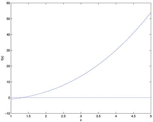
Figure 3.2

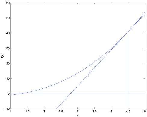
Figure 3.3

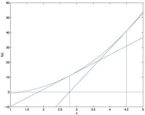
Figure 3.4

In the first illustration, we depict the graph of the function f along with the line y=0. The goal is to find a value of [latex]θ[/latex] such that [latex]f(θ)=0[/latex], and the solution is estimated to be around 1.3. Suppose we initialize the algorithm with [latex]θ=4.5[/latex], Newton’s method fits a straight line tangent to the function f at [latex]θ=4.5[/latex] and solves for the point where that line intersects the [latex]y=0[/latex] axis. This provides the next guess for [latex]θ[/latex], which is approximately 2.8. The subsequent illustration shows the outcome of an additional iteration, updating [latex]θ[/latex] to approximately 1.8. With a few more iterations, we quickly converge towards the final solution of [latex]θ=1.3[/latex].

Applying the same idea to maximize [latex]\ell(θ)[/latex], we would like to find the value of [latex]θ[/latex] that maximizes [latex]\ell(θ)[/latex]. Newton’s method can be applied here by considering the derivative of [latex]\ell(θ)[/latex] and using the above update rule. To be specific, given [latex]\ell(θ)[/latex], its derivative with respect to [latex]θ[/latex] can be computed, and Newton’s method can be applied by updating [latex]θ[/latex] as follows:

[latex]θ≔θ-\frac{\ell'θ}{\ell''θ}\tag{3.21}[/latex]

where [latex]\ell'(θ)[/latex] and [latex]\ell''(θ)[/latex]  are the first and second derivatives of [latex]\ell(θ)[/latex] with respect to [latex]θ[/latex], respectively. This process can be repeated until convergence. The advantage of this approach over gradient ascent is that Newton’s method converges much faster but requires the computation of the second derivative of [latex]\ell(θ)[/latex].

(Question: what if we would like to maximize instead of minimizing a function?)

The Newton-Raphson method is the generalization of Newton’s method to the multidimensional setting, which is necessary for our logistic regression setting where [latex]θ[/latex] is a vector. It is shown by:

[latex]θ≔θ-H^{-1}∇_θ\ell(θ)\tag{3.22}[/latex].

Where [latex]∇_θ\ell(θ)[/latex] is, as commonly, the vector representing the partial derivatives of [latex]\ell(θ)[/latex] with respect to the [latex]θ_i[/latex]‘s and [latex]H[/latex] is an n-by-n matrix (actually, n + 1-by-n + 1, assuming that we include the intercept term) called the Hessian, whose entries are given by

[latex]H_{ij}=\frac{∂^2\ell(θ)}{∂θ_i∂θ_j}.\tag{3.23}[/latex]

The generalization of Newton’s method, known as the Newton-Raphson method, can be applied to the logistic regression setting where [latex]θ[/latex] is a vector-valued parameter. This method typically converges faster and with fewer iterations compared to batch gradient descent. However, one iteration of Newton’s method can be more computationally expensive than one iteration of gradient descent, as it involves finding and inverting an [latex]n-[/latex]by[latex]-n[/latex] Hessian matrix. Nonetheless, if n is not too large, this method is usually much faster overall. When applied to maximize the logistic regression log likelihood function, [latex]\ell(θ)[/latex], the method is referred to as Fisher scoring.

Naive Bayes
To build an email spam filter using machine learning, we need to classify messages as either spam or non-spam. This type of problem is called text classification and is part of a larger set of challenges. After the learning process, the mail reader can automatically sort the spam messages into a separate folder. The feature vectors in this case are discrete-valued, unlike in gaussian discrimination analysis (GDA) where they were continuous and real-valued.

Representing an email might look like [latex]x=[0,0,0,1,0,1,1,...,0][/latex], (shown below) where the 1’s indicate the presence of certain words in the email, while the 0’s indicate the absence of those words. This representation of an email as a feature vector, where each feature represents the presence or absence of a specific word in the email, is commonly referred to as the “bag of words” representation. With this representation in hand, we can now use a machine learning algorithm to learn how to classify emails as either spam or non-spam based on their feature vectors. Specifically, if an email contains the i-th word of the dictionary, then we will set [latex]x_i=1[/latex]; otherwise, we let [latex]x_i[/latex] = 0. For instance, the vector

[latex]{\scriptsize x = \begin{bmatrix}1 \\ 0 \\ 0 \\ ⋮ \\ 1 \\ ⋮ \\ 0 \end {bmatrix} \begin{matrix}\textit{a} \\ \textit{vine} \\ \textit{group} \\ ⋮ \\ \textit{buy} \\ ⋮ \\ \textit{membership}\end {matrix}}[/latex]

is used to represent an email that contains the words “a” and “vine” but not “group,” “vine” or “membership.” The representation of an email as a feature vector, where the length of the feature vector is equal to the number of words in the dictionary, is a common approach in text classification problems like spam filtering. In this approach, the [latex]i[/latex]-th element of the feature vector is set to 1 if the email contains the [latex]i[/latex]-th word in the dictionary, and 0 otherwise. This feature vector is used to capture the presence or absence of words in an email. The set of words encoded in the feature vector is referred to as the vocabulary, and the dimension of the feature vector is equal to the size of the vocabulary.

Having chosen our feature vector, we now want to build a generative model. So, we have to model [latex]p(x|y)[/latex]. But if we have, say, a vocabulary of 50000 words, then [latex]x∈\{0;1\}^{50000}[/latex]([latex]x[/latex] is a 50000-dimensional vector of 0’s and 1’s), and if we were to model x explicitly with a multinomial distribution over the [latex]2^{50000}[/latex] possible outcomes, then we’d end up with a [latex](2^{50000}–1)[/latex] -dimensional parameter vector. This is clearly too many parameters.

To model [latex]p(x|y)[/latex], we will therefore make a very strong assumption. We will assume that the [latex]x_i[/latex]‘s are conditionally independent given [latex]y[/latex]. This assumption is called the Naive Bayes (NB) assumption, and the resulting algorithm is called the Naive Bayes classifier. For instance, if [latex]y=1[/latex] means spam email; “buy” is word 2087 and “price” is word 39831; then we are assuming that if I tell you [latex]y=1[/latex] (that a particular piece of email is spam), then knowledge of [latex]x_{2087}[/latex] (knowledge of whether “buy” appears in the message) will have no effect on your beliefs about the value of [latex]x_{39831}[/latex] (whether “price” appears). More formally, this can be written [latex]p(x_{2087}|y)=p(x_{2087}|y;x_{39831})[/latex]. (Note that this is not the same as saying that [latex]x_{2087}[/latex] and [latex]x_{39831}[/latex] are independent, which would have been written “[latex]p(x_{2087})=p(x_{2087}|x_{39831})[/latex]”; rather, we are only assuming that [latex]x_{2087}[/latex] and [latex]x_{39831}[/latex] are conditionally independent given [latex]y[/latex].)
We now have:

[latex]\begin{align*}p(x_{1},…,x_{50000}|y)&=p(x_1|y)p(x_2|y,x_1)p(x_3|y,x_1,x_2),…,p(x_{50000}|y,x_1,…,x_{49999})\\ &= p(x_1|y)p(x_2|y)p(x_3y),…,p(x_{50000}|y)\\ &= ∏_{i=1}^np(x_i|y) \tag{3.24}  \end{align*}[/latex]

The first equation is based on the fundamental principles of probabilities, while the second equation leverages the Naive Bayes assumption. Despite the fact that the Naive Bayes assumption is quite stringent, this algorithm has been observed to perform well on a variety of problems. Our model is parameterized by [latex]Φ_{i|y=1}=p(x_i=1|y=1),Φ_{i|y=0}=p(x_{i}=1|y=0)[/latex], and [latex]Φ_y=p(y=1)[/latex].
As usual, given a training set [latex]\{x^{(i)};y{(i)};i=1;…;m\}[/latex], we can write down the joint likelihood of the data:

[latex]\mathcal{L}(Φ_y,Φ_{j|y=0},Φ_{j|y=1})=∏_{i=1}^mp(x^{(i)}|y^{(i)}) \tag{3.25}[/latex].

Maximizing this with respect to [latex]Φ_y;Φ_{i|y=0}[/latex] and [latex]Φ_{i|y=1}[/latex] gives the maximum likelihood estimates:

[latex]Φ_{j|y=1}=\frac{∑_{i=1}^m1\bigl\{ x_j^{(i)}=1 ∧ y^{(i)}=1 \bigl\}}{∑_{i=1}^m1\{y^{(i)}=1\}}[/latex]

[latex]Φ_{j|y=0}=\frac{∑_{i=1}^m1\bigl\{ x_j^{(i)}=1 ∧ y^{(i)}=0 \bigl\}}{∑_{i=1}^m1\{y^{(i)}=0\}}[/latex]

[latex]Φ_{y}=\frac{∑_{i=1}^m 1\bigl\{y^{(i)}=1 \bigl\}}{m}\tag{3.26}[/latex]

The above equation involves the “and” symbol represented by the ” [latex]∧[/latex] ” symbol. The parameters in this equation have a clear interpretation, for example, [latex]Φ_{i|y=1}[/latex] represents the proportion of spam emails ([latex]y=1[/latex]) in which word j appears. To make a prediction on a new example with features [latex]x[/latex], we simply calculate the above expression as:

\begin{align} p(y=1|x) &=\frac{p(x|y=1)p(y=1)}{p(x)} \\ &= \frac{(\prod_{i=1}^np(x_i|y=1))p(y=1)}{(\prod_{i=1}^np(x_i|y=1))p(y=1) + (\prod_{i=1}^np(x_i|y=0))p(y=0)}\tag{3.27}\end{align} ,

and pick whichever class has the higher posterior probability.
Finally, it’s worth noting that although we have focused on the implementation of the Naive Bayes algorithm for binary-valued features, it can easily be adapted for cases where the [latex]x_i[/latex] can take on values from the set [latex]\{1,2,...,k_i\}[/latex]. In this scenario, [latex]p(x_i|y)[/latex] would be modeled as a multinomial distribution instead of a Bernoulli distribution. Additionally, even if some input features are originally continuous (such as the living area of a house), it’s common to convert them into a set of discrete values through discretization and apply the Naive Bayes algorithm. For example, the feature [latex]x_i[/latex] representing the living area of a house can be discretized by dividing the continuous values into the following ranges:

Thus, to apply the Naive Bayes algorithm to a house’s living area feature, we can convert the continuous value into a discrete one by discretizing it into a set of values. In this case, if a house has 890 square feet of living area, we set the corresponding feature value [latex]x_i[/latex] to 3. Then, we can model the probability [latex]p(x_i|y)[/latex] using a multinomial distribution instead of a Gaussian distribution. This approach is often better than using Gaussian Discriminant Analysis (GDA) when the original continuous features are not well modeled by a Gaussian distribution.

Laplace smoothing
In the Naive Bayes algorithm, 0 for both y = 0 (non-spam) and y = 1 (spam). However, now that you are getting emails containing the word “nips,” most of them are spam. The Naive Bayes algorithm therefore gets it completely wrong, because it gives [latex]p(y=1|x)=0[/latex] for all emails containing the word “nips.” This problem is known as the zero probability problem, and it arises because the Naive Bayes algorithm assigns a probability of zero to any event that was not seen in the training data.

The solution to the zero probability problem is simple: we add a small constant, typically one, to all entries of the [latex]Φ_{i|y}[/latex] matrices. This corresponds to adding Laplace smoothing to our estimate of the probabilities. This means that even if a word (or feature) does not appear in a class (spam or non-spam), we estimate its probability to be a small constant, rather than zero.

[latex]Φ_{35000|y=1}=\frac{∑_{i=1}^m1\bigl\{ x_35000^{(i)}=1 ∧ y^{(i)}=1 \bigl\}}{∑_{i=1}^m1\{y^{(i)}=1\}}=0[/latex]

[latex]Φ_{35000|y=0}=\frac{∑_{i=1}^m1\bigl\{ x_35000^{(i)}=1 ∧ y^{(i)}=0 \bigl\}}{∑_{i=1}^m1\{y^{(i)}=0\}}=0\tag{3.28}[/latex]

[latex]p(y=1|x)=p(y=0|x)=0[/latex]. This means that the algorithm has no information to make a prediction, so it gives equal probabilities for both classes (because it has never seen “nips” before in either spam or non-spam training examples). This problem is an example of zero probability or the problem of unseen features. To fix this, a common solution is to use Laplace (or add-k) smoothing, which adds a small constant k to each count, effectively avoiding the zero probability issue. The Laplace smoothed version of the estimate of the parameters is given by:

[latex]Φ_{i|y}=\frac{n_i+k}{n_y+k|V|}\tag{3.29}[/latex]

where [latex]n_i[/latex] is the number of times the i-th word appears in the emails of class [latex]y[/latex], [latex]n_y[/latex] is the number of emails in class [latex]y[/latex], [latex]k[/latex] is the smoothing constant, and [latex]|V|[/latex] is the size of the vocabulary.

While attempting to determine if one of these messages having “nips” is spam, it computes the class posterior probabilities, and attains

[latex]p(y=1|x) =\frac{(\prod_{i=1}^np(x_i|y=1))p(y=1)}{(\prod_{i=1}^np(x_i|y=1))p(y=1) + (\prod_{i=1}^np(x_i|y=0))p(y=0)}=\frac{0}{0}\tag{3.30}[/latex].

This is because each of the terms [latex]∏_{i=1}^np(x_i|y)[/latex] includes a term [latex]p(x_{35000}|y)=0[/latex] that is multiplied into it. Hence, our algorithm obtains 0=0, and doesn’t know how to make a prediction. Stating the problem more broadly, it is statistically a bad idea to estimate the probability of some event to be zero just because you haven’t seen it before in your finite training set. Take the problem of estimating the mean of a multinomial random variable z taking values in [latex]\{1;…;k\}[/latex]. We can parameterize our multinomial with [latex]Φ_i=p(z=i)[/latex]. Given a set of m independent observations [latex]\{z^{(1)};…;z^{(m)}\}[/latex], the maximum likelihood estimates are given by

[latex]Φ_j=\frac{∑_{i=1}^m1\{z^{(i)}=j\}}{m}\tag{3.31}[/latex].

As we saw previously, if we were to use these maximum likelihood estimates, then some of the [latex]Φ_j[/latex]‘s might end up as zero, which was a problem. To avoid this, we can use Laplace smoothing, which replaces the above estimate with

[latex]Φ_j=\frac{∑_{i=1}^m1\{z^{(i)}=j\}+1}{m+k}.\tag{3.32}[/latex]

Here, we’ve added 1 to the numerator, and k to the denominator. Note that [latex]∑_{j=1}^kΦ_j=1[/latex] still holds (check this yourself!), which is a desirable property since the [latex]Φ_j[/latex]‘s are estimates for probabilities that we know must sum to 1. Also, [latex]Φ_j≠0[/latex] for all values of [latex]j[/latex], solving our problem of probabilities being estimated as zero. Under certain (arguably quite strong) conditions, it can be shown that the Laplace smoothing actually gives the optimal estimator of the [latex]Φ_j[/latex]‘s. Returning to our Naive Bayes classifier, with Laplace smoothing, we therefore obtain the following estimates of the parameters:

[latex]Φ_{j|y=1}=\frac{∑_{i=1}^m1\bigl\{x_j^{(i)}=1∧y^{(i)}=1\bigl\}+1}{∑_{i=1}^m1\{y^{(i)}=1\}+2}[/latex]

[latex]Φ_{j|y=1}=\frac{∑_{i=1}^m1\bigl\{x_j^{(i)}=1∧y^{(i)}=0\bigl\}+1}{∑_{i=1}^m1\{y^{(i)}=0\}+2}\tag{3.33}[/latex]

(In practice, it usually doesn’t matter much whether we apply Laplace smoothing to [latex]Φ_y[/latex] or not, since we will typically have a fair fraction each of spam and non-spam messages, so [latex]Φ_y[/latex] will be a reasonable estimate of [latex]p(y=1)[/latex] and will be quite far from 0 anyway.)

Event models for text classification
To close of our discussion of generative learning algorithms, let’s talk about one more model that is specifically for text classification. While Naive Bayes as we’ve presented it will work well for many classification problems, for text classification, there is a related model that does even better. In the specific context of text classification, Naive Bayes as presented uses the what’s called the multivariate Bernoulli event model. In this model, we assumed that the way an email is generated is that first it is randomly determined (according to the class priors p (y)) whether a spammer or non-spammer will send you your next message. Then, the person sending the email runs through the dictionary, deciding whether to include each word i in that email independently and according to the probabilities [latex]p(x_i=1|y)=Φ_{i|y}[/latex]. Thus, the probability of a message was given by [latex]p(y)∏_{i=1}^np(x_i|y)[/latex].

Here’s a different model, called the multinomial event model. To describe this model, we will use a different notation and set of features for representing emails. We let [latex]x_i[/latex] denote the identity of the i-th word in the email. Thus, [latex]x_i[/latex] is now an integer taking values in [latex]\{1,…,|V_j\}[/latex], where [latex]|V|[/latex] is the size of our vocabulary (dictionary). An email of n words is now represented by a vector [latex](x_1,x_2,…,x_n)[/latex] of length [latex]n[/latex]; note that [latex]n[/latex]can vary for different documents. For instance, if an email starts with “A NIPS …,” then [latex]x_1=1[/latex] (“a” is the first word in the dictionary), and [latex]x_2=35000[/latex] (if “nips” is the 35000^th word in the dictionary). In the multinomial event model, we assume that the way an email is generated is via a random process in which spam/non-spam is first determined (according to [latex]p(y)[/latex]) as before. Then, the sender of the email writes the email by first generating [latex]x_1[/latex] from some multinomial distribution over words [latex](p(x_1|y))[/latex]. Next, the second word [latex]x_2[/latex] is chosen independently of [latex]x_1[/latex] but from the same multinomial distribution, and similarly for [latex]x_3,x_4[/latex], and so on, until all n words of the email have been generated. Thus, the overall probability of a message is given by [latex]p(y)∏_{i=1}^np(x_i|y)[/latex]. Note that this formula looks like the one we had earlier for the probability of a message under the multi-variate Bernoulli event model, but that the terms in the formula now mean very different things. In particular [latex]x_i|y[/latex] is now a multinomial, rather than a Bernoulli distribution.

The parameters for our new model are [latex]Φ_y=p(y)[/latex] as before, [latex]Φ_{k|y=1}=p(x_j=k|y=1)[/latex] (for any j) and [latex]Φ_{i|y=0}=p(x_j=k|y=0)[/latex]. Note that we have assumed that [latex]p(x_j|y)[/latex] is the same for all values of [latex]j[/latex] (i.e., that the distribution according to which a word is generated does not depend on its position [latex]j[/latex] within the email). If we are given a training set [latex]\{\left(x_i,y_i\right);i=1,…,m\}[/latex] where [latex]x^{(i)}= \left( x_1^{(i)},x_2^{(i)},…,x_{n_i}^{(i)}\right)[/latex](here, [latex]n_i[/latex] is the number of words in the i-training example), the likelihood of the data is given by

[latex]\mathcal{L}(Φ,Φ_{k|y=0},Φ_{k|y=1})=∏_{i=1}^mp(x^{(i)},y^{(i)})[/latex]

[latex]=∏_{i=1}^m\Bigl(∏_{j=1}^{n_i}p(x_j^{(i)}|y;Φ_{k|y=0},Φ_{k|y=1})\Bigl)p(y^{(i)};Φ_y). \tag{3.34}[/latex]

Maximizing this yields the maximum likelihood estimates of the parameters:

[latex]Φ_{k|y=1}=\frac{∑_{i=1}^m∑_{j=1}^{n_i}1\Bigl\{x_j^{(i)}=1∧y^{(i)}=1\Bigl\}}{∑_{i=1}^m1\{y^{(i)}=1\}n_i}[/latex]

[latex]Φ_{k|y=0}=\frac{∑_{i=1}^m∑_{j=1}^{n_i}1\Bigl\{x_j^{(i)}=1∧y^{(i)}=0\Bigl\}}{∑_{i=1}^m1\{y^{(i)}=0\}n_i}[/latex]

[latex]Φ_y=\frac{∑_{i=1}^m1\{y^{(i)}=1\}}{m}\tag{3.35}[/latex].

If we were to apply Laplace smoothing (which needed in practice for good performance) when estimating [latex]Φ_{k|y=0}[/latex] and [latex]Φ_{k|y=1}[/latex], we add 1 to the numerators and [latex]|V|[/latex] to the denominators, and obtain:

[latex]Φ_{k|y=1}=\frac{∑_{i=1}^m∑_{j=1}^{n_i}1\Bigl\{x_j^{(i)}=1∧y^{(i)}=1\Bigl\}+1}{∑_{i=1}^m1\{y^{(i)}=1\}n_i + |V|}[/latex]

[latex]Φ_{k|y=0}=\frac{∑_{i=1}^m∑_{j=1}^{n_i}1\Bigl\{x_j^{(i)}=1∧y^{(i)}=0\Bigl\}+1}{∑_{i=1}^m1\{y^{(i)}=0\}n_i + |V|}\tag{3.36}[/latex]

While not necessarily the very best classification algorithm, the Naive Bayes classifier often works surprisingly well. It is often also a very good “first thing to try,” given its simplicity and ease of implementation.

Support Vector Machines
This set of notes presents the Support Vector Machine (SVM) learning algorithm. SVMs are among the best (and many believe are indeed the best) “off-the-shelf” supervised learning algorithm. To tell the SVM story, we’ll need to first talk about margins and the idea of separating data with a large “gap.” Next, we’ll talk about the optimal margin classifier, which will lead us into a digression on Lagrange duality. We’ll also see kernels, which give a way to apply SVMs efficiently in very high dimensional (such as infinite-dimensional) feature spaces, and finally, we’ll close the story with the SMO algorithm, which gives an efficient implementation of SVMs.

Margins: Intuition
We’ll start our story on SVMs by talking about margins. This section will give the intuitions about margins and about the confidence of our predictions; these ideas will be made formal in “Functional and geometric margins”.
Consider logistic regression, where the probability [latex]p(y=1|x;θ)[/latex] is modeled by [latex]h_θ(x)=g(θ^Tx)[/latex]. We would then predict “1” on an input x if and only if [latex]h_θ(x)≥0.5[/latex], or equivalently, if and only if [latex]θ^Tx≥0[/latex]. Consider a positive training example (y = 1). The larger [latex]θ^Tx[/latex] is, the larger also is [latex]h_θ(x)=p(y=1|x;w,b)[/latex], and thus also the higher our degree of confidence that the label is 1. Thus, informally we can think of our prediction as being a very confident one that y = 1 if [latex]θ^Tx≫0[/latex]. Similarly, we think of logistic regression as making a very confident prediction of y = 0, if [latex]θ^Tx≪0[/latex]. Given a training set, again informally it seems that we’d have found a good fit to the training data if we can find θ so that [latex]θ^Tx_i≫0[/latex] whenever [latex]y_i=1[/latex], and [latex]θ^Tx_i≪0[/latex] whenever [latex]y_i=0[/latex], since this would reflect a very condent (and correct) set of classifications for all the training examples. This seems to be a nice goal to aim for, and we’ll soon formalize this idea using the notion of functional margins.

For a different type of intuition, consider the following figure, in which x’s represent positive training examples, o’s denote negative training examples, a decision boundary (this is the line given by the equation [latex]θ^Tx=0[/latex], and is also called the separating hyperplane) is also shown, and three points have also been labeled A, B and C.

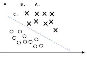
Figure 3.5

Notice that the point A is very far from the decision boundary. If we are asked to make a prediction for the value of y at A, it seems we should be quite condent that y = 1 there. Conversely, the point C is very close to the decision boundary, and while it’s on the side of the decision boundary on which we would predict y = 1, it seems likely that just a small change to the decision boundary could easily have caused our prediction to be y = 0. Hence, we’re much more confident about our prediction at A than at C. The point B lies in-between these two cases, and more broadly, we see that if a point is far from the separating hyperplane, then we may be significantly more confident in our predictions. Again, informally we think it’d be nice if, given a training set, we manage to find a decision boundary that allows us to make all correct and confident (meaning far from the decision boundary) predictions on the training examples. We’ll formalize this later using the notion of geometric margins.

To make our discussion of SVMs easier, we’ll first need to introduce a new notation for talking about classification. We will be considering a linear classifier for a binary classification problem with labels y and features x. From now, we’ll use [latex]y∈{-1;1}[/latex] (instead of [latex]\{0;1\}[/latex]) to denote the class labels. Also, rather than parameterizing our linear classifier with the vector [latex]θ[/latex], we will use parameters [latex]\textbf{w;b}[/latex], and write our classifier as

[latex]h_{w,b}(x) = g(w^Tx+b)\tag{3.37}[/latex].

Here, [latex]\textbf{g}(\textbf{z})=1[/latex] if [latex]\textbf{z}≥0[/latex], and [latex]\textbf{g}(\textbf{z})=-1[/latex] otherwise. This [latex]\textbf{w};\textbf{b}[/latex] notation allows us to explicitly treat the intercept term [latex]\textbf{b}[/latex] separately from the other parameters. (We also drop the convention we had previously of letting [latex]\textbf{x}_0=1[/latex] be an extra coordinate in the input feature vector.) Thus, b takes the role of what was previously [latex]\textbf{θ}_0[/latex], and [latex]\textbf{w}[/latex] takes the role of [latex][\textbf{θ}1…\textbf{θ}n]^T[/latex].

Note also that, from our definition of g above, our classifier will directly predict either 1 or –1 (cf. the perceptron algorithm), without first going through the intermediate step of estimating the probability of y being 1 (which was what logistic regression did).

Functional and geometric margins
Let’s formalize the notions of the functional and geometric margins. Given a training example x(i); y(i), we define the functional margin of (w; b) with respect to the training example

[latex]γ̂^{(i)}=y^{(i)}(w^Tx+b) \tag{3.38}[/latex].

Note that if [latex]y^{(i)}=1[/latex], then for the functional margin to be large (i.e., for our prediction to be condent and correct), we need [latex]w^Tx+b[/latex] to be a large positive number. Conversely, if [latex]y^{(i)}=-1[/latex], then for the functional margin to be large, we need [latex]w^Tx+b[/latex] to be a large negative number. Moreover, if [latex]y^{(i)}(w^Tx+b)>0[/latex], thenour prediction on this example is correct. (Check this yourself.) Hence, a large functional margin represents a confident and a correct prediction.

For a linear classifier with the choice of g given above (taking values in [latex]-1;1[/latex] ), there’s one property of the functional margin that makes it not a very good measure of confidence, however. Given our choice of [latex]g[/latex], we note that if we replace [latex]w[/latex] with 2w and b with 2b, then since [latex]g(w^Tx+b)=g(2w^Tx+2b)[/latex], this would not change [latex]h_{w,b}(x)[/latex] at all. I.e., g, and hence also [latex]h_{w,b}(x)[/latex], depends only on the sign, but not on the magnitude, of [latex]w^Tx+b[/latex]. However, replacing [latex](w,b)[/latex] with [latex](2w,2b)[/latex] also results in multiplying our functional margin by a factor of 2. Thus, it seems that by exploiting our freedom to scale w and b, we can make the functional margin arbitrarily large without really changing anything meaningful. Intuitively, it might therefore make sense to impose some sort of normalization condition such as that [latex]||w||_2=1[/latex]; i.e., we might replace [latex](w,b)[/latex] with [latex](w/||w||_2,b/||w||_2)[/latex], and instead consider the functional margin of  [latex](w/||w||_2,b/||w||_2)[/latex]. We’ll come back to this later.

Given a training set [latex]S=\{(x^{(i)},y^{(i)});i=1,…,m \}[/latex], we also define the function margin of [latex](w,b)[/latex] with respect to S to be the smallest of the functional margins of the individual training examples. Denoted by [latex]γ̂[/latex], this can therefore be written:

[latex]γ̂^{(i)}=\min\limits_{i=1,\dots,m} γ̂^{(i)}\tag{3.39}[/latex].

Next, let’s talk about geometric margins. Consider the picture below:

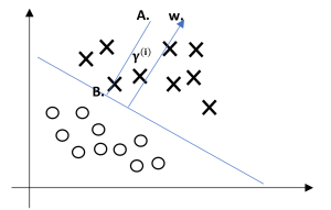
Figure 3.6

The decision boundary corresponding to (w; b) is shown, along with the vector w. Note that w is orthogonal (at 90°◦) to the separating hyperplane. (You should convince yourself that this must be the case.) Consider the point at A, which represents the input [latex]x^{(i)}[/latex] of some training example with label [latex]y^{(i)}[/latex]= 1. Its distance to the decision boundary,[latex]γ^{(i)}[/latex], is given by the line segment AB.
How can we find the value of [latex]γ^{(i)}[/latex]? Well, [latex]w/||w||[/latex] is a unit-length vector pointing in the same direction as w. Since A represents [latex]x^{(i)}[/latex], we therefore find that the point B is given by [latex]x^{(i)}-y^{(i)} \cdot w/||w||[/latex]. But this point lies on the decision boundary, and all points x on the decision boundary satisfy the equation [latex]w^Tx+b=0[/latex]. Hence,

[latex]w^T(x^{(i)}-γ^{(i)}\frac{w}{||w||})+b=0. \tag{3.40}[/latex]

Solving for [latex]γ^{(i)}[/latex] yields

[latex]γ^{(i)} = \frac{w^Tx^{(i)}+b}{||w||}=\left( \frac{w}{||w||}\right)^Tx^{(i)}+\frac{b}{||w||}. \tag{3.41}[/latex]

This was worked out for the case of a positive training example at A in the figure, where being on the positive side of the decision boundary is good. More generally, we define the geometric margin of (w; b) with respect to a training example [latex]x^{(i)},y^{(i)}[/latex] to be

[latex]γ^{(i)} = y^{(i)} \left( \left(\frac{w}{||w||}\right)^Tx^{(i)}+\frac{b}{||w||}\right).\tag{3.42}[/latex]

Note that if [latex]||w||=1[/latex], then the functional margin equals the geometric margin this thus gives us a way of relating these two different notions of margin. Also, the geometric margin is invariant to rescaling of the

[latex]γ = \min\limits_{i=1,\dots,m} γ^{(i)}\tag{3.43}[/latex]

The optimal margin classifier
Given a training set, it seems from our previous discussion that a natural desideratum is to try to find a decision boundary that maximizes the (geometric) margin, since this would reflect a very confident set of predictions on the training set and a good fit to the training data. Specifically, this will result in a classifier that separates the positive and the negative training examples with a gap (geometric margin).
For now, we will assume that we are given a training set that is linearly separable; i.e., that it is possible to separate the positive and negative examples using some separating hyperplane. How we find the one that achieves the maximum geometric margin? We can pose the following optimization problem:

[latex]\begin{aligned} \text{max}_{γ,w,b} \quad  & \quad \quad \quad \quad \quad \quad \quad γ \\ \textrm{s.t.} \quad & y^{(i)}(w^Tx^{(i)}+b) \geq  γ, \quad i = 1,\dots, m \\ & \quad \quad \quad \quad \quad||w|| = 1. \\ \end{aligned}\tag{3.44}[/latex]

I.e., we want to maximize γ, subject to each training example having functional margin at least γ. The [latex]||w||=1[/latex] constraint moreover ensures that the functional margin equals to the geometric margin, so we are also guaranteed that all the geometric margins are at least γ. Thus, solving this problem will result in (w; b) with the largest possible geometric margin with respect to the training set.
If we could solve the optimization problem above, we’d be done. But the [latex]||w||=1[/latex] constraint is a nasty (non-convex) one, and this problem certainly isn’t in any format that we can plug into standard optimization software to solve. So, let’s try transforming the problem into a nicer one. Consider:

[latex]\begin{aligned} \text{max}_{γ,w,b} \quad  & \quad \quad \quad \quad \quad \quad \frac{γ̂}{||w||} \\ \textrm{s.t.} \quad & y^{(i)}(w^Tx^{(i)}+b) \geq  γ̂, \quad i = 1,\dots, m  \\ \end{aligned}\tag{3.45}[/latex]

Here, we’re going to maximize [latex]\frac{γ̂}{||w||}[/latex], subject to the functional margins all being at least [latex]γ̂[/latex]. Since the geometric and functional margins are related by [latex]γ=\frac{γ̂}{||w||}[/latex], this will give us the answer we want. Moreover, we’ve gotten rid of the constraint [latex]||w||=1[/latex] that we didn’t like. The downside is that we now have a nasty (again, non-convex) objective [latex]\frac{γ̂}{||w||}[/latex] function; and, we still don’t have any off-the-shelf software that can solve this form of an optimization problem.
Let’s keep going. Recall our earlier discussion that we can add an arbitrary scaling constraint on w and b without changing anything. This is the key idea we’ll use now. We will introduce the scaling constraint that the functional margin of w; b with respect to the training set must be 1:

[latex]γ̂=1.[/latex]

Since multiplying w and b by some constant results in the functional margin being multiplied by that same constant, this is indeed a scaling constraint, and can be satisfied by rescaling w; b. Plugging this into our problem above, and noting that maximizing [latex]\frac{γ̂}{||w||}[/latex] = [latex]\frac{1}{||w||}[/latex] is the same thing as minimizing [latex]||w||^2[/latex], we now have the following optimization problem:

[latex]\begin{aligned} \text{max}_{γ,w,b} \quad  & \quad \quad \quad \quad \quad \quad \frac{1}{2}||w||^2 \\ \textrm{s.t.} \quad & y^{(i)}(w^Tx^{(i)}+b) \geq  1, \quad i = 1,\dots, m  \\ \end{aligned}\tag{3.46}[/latex]

We’ve now transformed the problem into a form that can be efficiently solved. The above is an optimization problem with a convex quadratic objective and only linear constraints. Its solution gives us the optimal margin classifier. This optimization problem can be solved using commercial quadratic programming (QP) code. While we could call the problem solved here, what we will instead do is make a digression to talk about Lagrange duality. This will lead us to our optimization problem’s dual form, which will play a key role in allowing us to use kernels to get optimal margin classifiers to work efficiently in very high dimensional spaces.

Optimal margin classifiers
Previously, we posed the following (primal) optimization problem for finding the optimal margin classifier:

[latex]\begin{aligned} \text{min}_{γ,w,b} \quad  & \quad \quad \quad \quad \quad \quad \frac{1}{2}||w||^2 \\ \textrm{s.t.} \quad & y^{(i)}(w^Tx^{(i)}+b) \geq  1, \quad i = 1,\dots, m  \\ \end{aligned}[/latex]

We can write the constraints as

[latex]g_{i(w)}=-y^{(i)}(w^Tx^{(i)}+b)+1≤0 \tag{3.47}[/latex].

We have one such constraint for each training example. Note that from the KKT (Karush-Kuhn-Tucker (KKT) conditions) dual complementarity condition, we will have [latex]α_i>0[/latex] only for the training examples that have functional margin exactly equal to one (i.e., the ones corresponding to constraints that hold with equality, [latex]g_i(w)=0[/latex]). Consider the figure below, in which a maximum margin separating hyperplane is shown by the solid line.

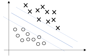
Figure 3.7

The points with the smallest margins are exactly the ones closest to the decision boundary; here, these are the three points (one negative and two positive examples) that lie on the dashed lines parallel to the decision boundary. Thus, only three of the [latex]α_i[/latex]‘s, namely the ones corresponding to these three training examples, will be non-zero at the optimal solution to our optimization problem. These three points are called the support vectors in this problem. The fact that the number of support vectors can be much smaller than the size the training set will be useful later.

Let’s move on. Looking ahead, as we develop the dual form of the problem, one key idea to watch out for is that we’ll try to write our algorithm in terms of only the inner product [latex]\text{<}x^{(i)},x^{(j)}\text{>}[/latex] (think of this as [latex]((x^{(i)})^T,x^{(j)})[/latex] between points in the input feature space. The fact that we can express our algorithm in terms of these inner products will be key when we apply the kernel trick.
When we construct the Lagrangian for our optimization problem we have:

[latex]\mathcal{L}(w,b,α) = \frac{1}{2}||w||^2 - \sum_{i=1}^m a_i [y^{(i)} (w^T x^{(i)} + b) - 1]. \tag{3.48}[/latex]

Note that there’re only [latex]α_{i}[/latex] but no [latex]β_i[/latex] Lagrange multipliers, since the problem has only inequality constraints. Let’s find the dual form of the problem. To do so, we need to first minimize [latex]\mathcal{L}(w,b,α)[/latex] with respect to [latex]w[/latex]  and b (for fixed α), to get [latex]\textbf{θ}_D[/latex], which we’ll do by setting the derivatives of [latex]\mathcal{L}[/latex] with respect to w and b to zero.
We have:

[latex]\nabla_w \mathcal{L} (w,b,α) = w -\sum_{i=1}^m α_i y^{(i)} x^{(i)} = 0[/latex]

This implies that

[latex]w = \sum_{i = 1}^m α_i y^{(i)} x^{(i)} \tag{3.49}[/latex]

As for the derivative with respect to b, we obtain

[latex]\frac{∂}{∂b}\mathcal{L}(w,b,α) = \sum_{i = 1}^m α_iy^{(i)}=0. \tag{3.50}[/latex]

If we take the definition of w in Equation (3.49) and plug that back into the Lagrangian (Equation (3.48)), and simplify, we get

[latex]\mathcal{L}(w,b,α) = \sum_{i=1}^m α_i - \frac{1}{2} \sum_{i,j=1}^m y^{(i)} y^{(j)} α_i α_j (x^{(i)})^Tx^{(j)}-b\sum_{i=1}^m α_i y^{(i)}.\tag{3.51}[/latex]

But from Equation this equation, the last term must be zero, so we obtain.

[latex]\mathcal{L}(w,b,α) = \sum_{i=1}^m α_i -\frac{1}{2}\sum_{i,j=1}^m y^{(i)} y^{(j)}α_i α_j (x^{(i)})^Tx^{(j)}.\tag{3.52}[/latex]

Recall that we got to the equation above by minimizing L with respect to w and b. Putting this together with the constraints [latex]α_i\geq0[/latex] (that we always had) and the constraint (3.50), we obtain the following dual optimization problem:

[latex]\begin{aligned} \text{max}_{α} \quad  & W(α) = \sum_{i=1}^m α_i - \frac{1}{2}\sum_{i,j=1}^m y^{(i)} y^{(j)} a_i a_j \left< x^{(i)}, x^{(j)} \right>\ .  \\ \textrm{s.t.} \quad &  \quad \quad \quad \quad \quad \quad α_i \geq  0, \quad i = 1,\dots, m \\ & \quad \quad \quad \quad \quad \quad \quad\sum_{i=1}^m α_i y^{(i)} = 0, \\ \end{aligned}\tag{3.53}[/latex]

You should also be able to verify the KKT conditions to hold are indeed satisfied in our optimization problem. Hence, we can solve the dual in lieu of solving the primal problem. Specifically, in the dual problem above, we have a maximization problem in which the parameters are the [latex]α_i[/latex]‘s. We’ll talk later about the specific algorithm that we’re going to use to solve the dual problem, but if we are indeed able to solve it (i.e., find the α‘s that maximize [latex]W(α)[/latex] subject to the constraints), then we can use Equation (3.49) to go back and find the optimal w‘s as a function of the α‘s. Having found [latex]w^*[/latex], by considering the primal problem, it is also straightforward to find the optimal value for the intercept term b as

[latex]b^* = -\frac{max_{i:y^{(i)}=-1} w^{*T}x^{(i)} + min_{i:y^{(i)}=1}w^{*T}x^{(i)}}{2}\tag{3.54}[/latex]

(Check for yourself that this is correct.)

Before moving on, let’s also take a more careful look at Equation (3.49), which gives the optimal value of w in terms of (the optimal value of) [latex]α[/latex]. Suppose we’ve t our model’s parameters to a training set, and now wish to make a prediction at a new point input x. We would then calculate [latex]w^Tx+b[/latex], and predict y = 1 if and only if this quantity is bigger than zero. But using (3.49), this quantity can also be written:

[latex]\begin{align*} w^Tx+b &= \left( \sum_{i=1}^m α_i y^{(i)} x^{(i)}\right)^T x+b \\ &= \sum_{i = 1}^m α_i y^{(i)} \left< x^{(i)} , x \right> + b.  \end{align*}\tag{3.55}[/latex]

Hence, if we’ve found the [latex]α_i[/latex]‘s, in order to make a prediction, we have to calculate a quantity that depends only on the inner product between x and the points in the training set. Moreover, we saw earlier that the [latex]α_i[/latex]‘s will all be zero except for the support vectors. Thus, many of the terms in the sum above will be zero, and we really need to find only the inner products between x and the support vectors (of which there is often only a small number) in order calculate (3.55) and make our prediction. By examining the dual form of the optimization problem, we gained significant insight into the structure of the problem, and were also able to write the entire algorithm in terms of only inner products between input feature vectors. In the next section, we will exploit this property to apply the kernels to our classification problem. The resulting algorithm, support vector machines, will be able to efficiently learn in very high dimensional spaces.

Source: Machine Learning (Course). Andrew Ng. Openstax CNX (Rice University) 2013. https://cnx.org/contents/THQBCjjQ@4.2:AifRdKFz@2/Machine-Learning-Introduction