Introduction to Regression Analysis

Regression analysis is a fundamental technique in machine learning that aims to model and understand the relationship between variables. It provides a framework for predicting continuous outcomes based on input features. This powerful tool allows us to uncover patterns, make inferences, and make informed decisions in various fields such as economics, finance, healthcare, and social sciences. At its core, regression analysis seeks to estimate the parameters of a mathematical model that best describes the relationship between the dependent variable (the outcome to be predicted) and independent variables (the features that influence the outcome). The ultimate goal is to create a model that can accurately predict the outcome of new, unseen data. One of the commonly used regression methods is linear regression, which assumes a linear relationship between the independent variables and the dependent variable. It estimates the coefficients that define the linear equation, aiming to minimize the difference between the predicted values and the actual observations. Linear regression provides interpretable insights into how each independent variable contributes to the outcome and allows for easy inference.

However, not all relationships in the real world are linear. In such cases, more advanced regression techniques come into play. Polynomial regression, for instance, can capture non-linear relationships by introducing higher-order terms to the linear equation. This flexibility enables the model to capture complex patterns and improve prediction accuracy. Moreover, regression analysis extends beyond single-variable predictions. Multiple regression incorporates multiple independent variables to account for their combined effect on the outcome. This approach enables us to explore the interplay between various factors and gain a deeper understanding of their impact.

In addition to traditional regression methods, machine learning offers sophisticated algorithms like decision trees, random forests, support vector regression, and neural networks. These models can capture intricate relationships and handle large-scale datasets with high dimensionality. The process of regression analysis involves several steps. It begins with data preprocessing, including cleaning, normalization, and feature engineering to ensure the input variables are suitable for analysis. Next, the model is trained using a training dataset, where the algorithm learns the underlying patterns and adjusts its parameters to minimize prediction errors. To evaluate the performance of the regression model, various metrics are used, such as mean squared error (MSE), root mean squared error (RMSE), and coefficient of determination (R-squared). These metrics assess the accuracy and goodness of fit of the model to the observed data.

Regression analysis also enables us to assess the statistical significance of the estimated coefficients and conduct hypothesis tests. This provides insights into the significance of each independent variable in influencing the outcome. It is a powerful tool in machine learning that allows us to model and predict continuous outcomes based on input features. It provides valuable insights into the relationship between variables and helps make informed decisions in various domains. By leveraging regression techniques, we can uncover patterns, understand complex relationships, and make accurate predictions to drive advancements in numerous fields.

Supervised learning

Let’s start by talking about a few examples of supervised learning problems. Suppose we have a dataset giving the different types of vehicles and mile-per-gallon and other features of the cars are represented as below:

Table 2.1

We can plot this data:

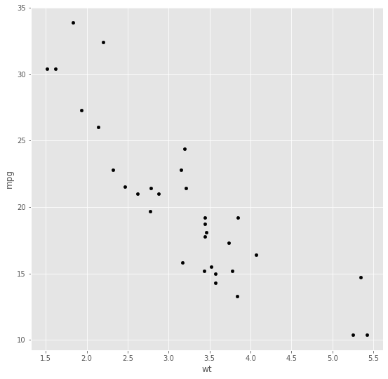
Figure 2.1

Given data like this, how can we learn to predict the MPG with respect to the weight of the cars, as a function of the weight MPG?
To establish a notation for future use, we’ll use [latex]x^{(i)}[/latex]to denote the “input” variables (living area in this example), also called input features, and [latex]y^{(i)}[/latex]to denote the “output” or target variable that we are trying to predict (price). A pair [latex](x^{(i)},y^{(i)})[/latex]is called a training example, and the dataset that we’ll be using to learn a list of [latex]m[/latex] training examples [latex]\{{(x^{(i)},y^{(i)} ); i=1,…,m}\}[/latex]– is called a training set. Note that the superscript “[latex](i)[/latex]” in the notation is simply an index into the training set and has nothing to do with exponentiation. We will also use [latex]X[/latex] denote the space of input values, and [latex]Y[/latex] the space of output values. In this example, [latex]X=Y=\mathbb{R}[/latex]. To describe the supervised learning problem slightly more formally, our goal is, given a training set, to learn a function [latex]h:X→Y[/latex] so that [latex]h(x)[/latex] is a “good” predictor for the corresponding value of . For historical reasons, this function [latex]h[/latex] is called a hypothesis. Seen pictorially, the process is therefore like this:

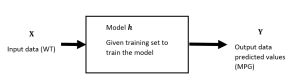
Figure 2.2

When the target variable that we’re trying to predict is continuous, such as in our cars example, we call the learning problem a regression problem. When [latex]y[/latex] can take on only a small number of discrete values (such as if, given the car weight, we wanted to predict MPG rate), we call it a classification problem.

Linear Regression

To make our cars example more interesting, let’s consider a slightly richer dataset in which we also know the horsepower (HP) of each car:

Table 2.2

Here, the [latex]x[/latex] ‘s are two-dimensional vectors in [latex]\mathbb{R}^2[/latex]. For instance, [latex]x_1^{(i)}[/latex] is the [latex]i[/latex]-th car in the training set, and [latex]x_2^{(i)}[/latex] is its HP. (In general, when designing a learning problem, it will be up to you to decide what features to choose you might also decide to include other features such as car’s cylinders, and so on. We’ll say more about feature selection later, but for now let’s take the features as given.) 
To perform supervised learning, we must decide how we’re going to represent functions hypotheses [latex]h[/latex] in a computer. As an initial choice, let’s say we decide to approximate [latex]y[/latex] as a linear function of [latex]x[/latex]:

Here, the [latex]θ_i[/latex]‘s are the parameters (also called weights) parameterizing the space of linear functions mapping from [latex]X[/latex] to [latex]Y[/latex]. When there is no risk of confusion, we will drop the [latex]θ[/latex] subscript in [latex]h_θ(x)[/latex], and write it more simply as [latex]h(x)[/latex]. To simplify our notation, we also introduce the convention of letting [latex]x_0=1[/latex] (this is the intercept term), so that

[latex]h(x)= ∑_{i=0}^{n} θ_i x_i= θ^{T}\tag{2.2}[/latex]

where on the right-hand side above we are viewing [latex]θ[/latex] and [latex]x[/latex] both as vectors, and here [latex]n[/latex] is the number of input variables (not counting [latex]x_0[/latex]). Now, given a training set, how do we pick, or learn, the parameters [latex]θ[/latex]? One reasonable method seems to be to make [latex]h(x)[/latex] close to [latex]y[/latex], at least for the training examples we have. To formalize this, we will dene a function that measures, for each value of the [latex]θ[/latex]‘s, how close the [latex]h(x^{(i)})[/latex]‘s are to the corresponding [latex]y^{(i)}[/latex]‘s. We dene the cost function:

[latex]J(θ)=1/2 ∑_{(i=1)}^{m} (h_θ (x^{(i)} )-y^{(i)} )^{2}.\tag{2.3}[/latex]

If you’ve seen linear regression before, you may recognize this as the familiar least-squares cost function that gives rise to the ordinary least-squares regression model. Whether or not you have seen it previously, let’s keep going, and we’ll eventually show this to be a special case of a much broader family of algorithms.

LMS algorithm

We want to choose [latex]θ[/latex]  so as to minimize [latex]J(θ)[/latex]. To do so, let’s use a search algorithm that starts with some initial guess for [latex]θ[/latex], and that repeatedly changes [latex]θ[/latex] to make [latex]J(θ)[/latex] smaller, until hopefully, we converge to a value of [latex]θ[/latex] that minimizes [latex]J(θ)[/latex]. Specifically, let’s consider the gradient descent algorithm, which starts with some initial [latex]θ[/latex], and repeatedly performs the update:

[latex]θ_j≔θ_j-α \frac{∂}{∂θ_j} J(θ).\tag{2.4}[/latex]

(This update is simultaneously performed for all values of [latex]j=0,…,n[/latex].) Here, [latex]α[/latex] is called the learning rate. This is a very natural algorithm that repeatedly takes a step in the direction of the steepest decrease of [latex]J[/latex]. In order to implement this algorithm, we have to work out what is the partial derivative term on the right-hand side. Let’s rst work it out for the case of if we have only one training example [latex](x;y)[/latex], so that we can neglect the sum in the definition of [latex]J[/latex]. We have:

[latex]\begin{align*}\frac{∂}{∂θ_j} J(θ) &= \frac{∂}{∂θ_j} \frac{1}{2} (h_θ (x)-y)^{2}\\ &=2 \cdot \frac{1}{2} (h_θ (x)-y)\cdot \frac{∂}{∂θ_j } (h_θ (x)-y)\\ &=(h_θ (x)-y)\cdot \frac{∂}{∂θ_j} (∑_{i=0}^{n} θ_i x_i-y)\\ &= (h_θ (x)-y) x_j\tag{2.5}\end{align*}[/latex]

For a single training example, this gives the update rule:

[latex]θ_j≔θ_j+α(y^{(i)}-h_θ (x^{(i)}))x_j^{(i)}.\tag{2.6}[/latex].

The rule is called the LMS update rule (LMS stands for least mean squares) and is also known as the Widrow-Hoff learning rule. This rule has several properties that seem natural and intuitive. For instance, the magnitude of the update is proportional to the error term [latex](y^{(i)} -h_θ (x^{(i)}))[/latex] thus, for instance, if we are encountering a training example in which our prediction nearly matches the actual value of [latex]y^{(i)}[/latex], then we nd that there is little need to change the parameters; in contrast, a larger change to the parameters will be made if our prediction [latex]h_θ (x^{(i)})[/latex] has a large error (i.e., if it is very far from [latex]y^{(i)}[/latex]). 
We have derived the LMS rule for when there was only a single training example. There are two ways to modify this method for a training set of more than one example. The rest is replaced it with the following algorithm:

• Repeat until converge{
  • [latex]θ_j≔θ_j+α∑_{i=1}^{m}(y^{(i)}-h_θ (x^{(i)})) x_j^{(i)}[/latex] (for every j).
    
• }

The reader can easily verify that the quantity in the summation in the update rule above is just [latex]\frac{∂}{∂θ_j} J(θ)[/latex] (for the original definition of [latex]J[/latex]). So, this is simply gradient descent on the original cost function [latex]J[/latex]. This method looks at every example in the entire training set on every step and is called batch gradient descent. Note that, while gradient descent can be susceptible to local minima in general, the optimization problem we have posed here for linear regression has only one global, and no other local, optima; thus gradient descent always converges (assuming the learning rate [latex]α[/latex] is not too large) to the global minimum. Indeed, [latex]J[/latex] is a convex quadratic function. Here is an example of gradient descent as it is run to minimize a quadratic function.

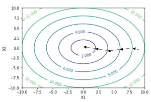
Figure 2.3

The ellipses shown above are the contours of a quadratic function. Also shown is the trajectory taken by gradient descent, which was initialized at (48,30). The [latex]x[/latex] ‘s in the figure (joined by straight lines) mark the successive values of [latex]θ[/latex] that gradient descent went through.

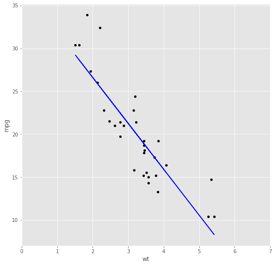
Figure 2.4

When we run batch gradient descent to t θ on our previous dataset, to learn to predict housing price as a function of living area, we obtain [latex]θ_0[/latex] = 37.28, [latex]θ_1[/latex] = -5.34. If we plot [latex]h_θ (x)[/latex] as a function of [latex]x[/latex] (area), along with the training data, we obtain the following figure:

• Repeat until converge {
  • For i=1 to m, {
    • [latex]θ_j≔θ_j+α∑_{i=1}^{m} (y^{(i)}-h_θ (x^{(i)})) x_j^{(i)}[/latex] (for every j).
  • }
• }

In this algorithm, we repeatedly run through the training set, and each time we encounter a training example, we update the parameters according to the gradient of the error with respect to that single training example only. This algorithm is called stochastic gradient descent (also incremental gradient descent). Whereas batch gradient descent has to scan through the entire training set before taking a single step a costly operation if [latex]m[/latex] is large stochastic gradient descent can start making progress right away and continues to make progress with each example it looks at. Often, stochastic gradient descent gets [latex]θ[/latex] close to the minimum much faster than batch gradient descent. (Note however that it may never converge to the minimum, and the parameters [latex]θ[/latex] will keep oscillating around the minimum of [latex]J(θ)[/latex]; but in practice most of the values near the minimum will be reasonably good approximations to the true minimum. For these reasons, particularly when the training set is large, stochastic gradient descent is often preferred over batch gradient descent.

Python Implementation

Here is how to implement linear regression in the different forms in Python.

import numpy as np
import pandas as pd
import matplotlib
import matplotlib.pyplot as plt

# Load mtcars data set
mtcars = pd.read_csv(“C:/Users/bardi/Documents/Python Scripts/ENBC311/mtcars.csv”)

mtcars.plot(kind=“scatter”, x=”wt”, y=“mpg”, figsize=(8,8), color=“black”)

This code creates scatter plot indicating the data points in the space. We are going to use scikit-learn library with the wide range of different ML functions to create linear regression;

from sklearn import linear_model

# Initialize model
regression_model = linear_model.LinearRegression()

# Train the model using the mtcars data
regression_model.fit(X = pd.DataFrame(mtcars[“wt”]), y = mtcars[“mpg”])

# Check trained model y-intercept
print(regression_model.intercept_)

# Check trained model coefficients
print(regression_model.coef_)

The normal equations
Gradient descent gives one way of minimizing [latex]J[/latex]. Let’s discuss a second way of doing so, this time performing the minimization explicitly and without resorting to an iterative algorithm. In this method, we will minimize [latex]J[/latex] by explicitly taking its derivatives with respect to the [latex]θ_j[/latex] ‘s, and setting them to zero. To enable us to do this without having to write reams of algebra and pages full of matrices of derivatives, let’s introduce some notations for doing calculus with matrices.

Matrix derivatives

For a function [latex]f: \mathbb{R}^{(m×n)}→ \mathbb{R}[/latex] mapping from m-by-n matrices to the real numbers, we define the derivative of [latex]f[/latex] with respect to [latex]A[/latex] to be:

Thus, the gradient [latex]∇_A f(A)[/latex] is itself an m-by-n matrix, whose [latex](i; j)[/latex]-element is [latex]\frac{∂f}{∂A_{ij}}[/latex]. For example, suppose [latex]{\scriptstyle A= \begin{bmatrix}A_{11}&A_{12} \\ A_{21} & A_{22} \end{bmatrix}}[/latex] is a 2-by-2 matrix, and the function [latex]f: \mathbb{R}^{(2×2)}→ \mathbb{R}[/latex] is given by

[latex]f(A) = \frac{3}{2}A_{11} + 5A_{12}^{2}+A_{21}A_{22}[/latex].

Here, [latex]A_{ij}[/latex]  denotes the [latex](i,j)[/latex]  entry of the matrix [latex]A[/latex]. We then have

[latex]∇_A f(A)= \begin{bmatrix}\frac{3}{2}&10A_{12}\\A_{22} & A_{21} \end{bmatrix}[/latex].

We also introduce the trace operator, written “tr.” For an n-by-n (square) matrix [latex]A[/latex], the trace of [latex]A[/latex]  is defined to be the sum of its diagonal entries:

[latex]\sum_{i=1}^n A_{ii}\tag{2.10}[/latex]

If a is a real number (i.e., a 1-by-1 matrix), then [latex]tr \text{ } a = a[/latex]. (If you haven’t seen this “operator notation”before, you should think of the trace of [latex]A[/latex] as [latex]tr(A)[/latex], or as application of the “trace” function to the matrix . It’s more commonly written without the parentheses, however.)
The trace operator has the property that for two matrices [latex]A[/latex] and [latex]B[/latex] such that [latex]AB[/latex] is square, we have that [latex]trAB=trBA[/latex]. (Check this yourself!) As corollaries of this, we also have, e.g.,

[latex]\text{trABC = trCAB = trBCA}[/latex]

[latex]\text{trABCD = trDABC = trCDAB = trBCDA.}\tag{2.11}[/latex]

The following properties of the trace operator are also easily verified. Here, A and B are square matrices, and a is a real number:

[latex]\text{trA=trA}^{\text{T}}[/latex]

[latex]\text{tr(A+B)=trA+trB}[/latex]

[latex]\text{tr aA=a trA}\tag{2.12}[/latex]

We now state without proof some facts of matrix derivatives (we won’t need some of these until later this quarter). (2.13) applies only to non-singular square matrices A, where |A|denotes the determinant of A. We have:

[latex]∇_{\text{A}}\text{trAB = B}^\text{T}[/latex]

[latex]\text{∇}_{\text{A}^{T}}\text{f(A) = (∇}_{\text{A}}\text{f(A}\text{)})^{\text{T}}[/latex]

[latex]∇_{\text{A}}\text{trABA}^{\text{T}}\text{C = CAB} + \text{C}^\text{T}AB^\text{T}[/latex]

[latex]∇_{\text{A}}|\text{A}|\text{ = }|\text{A}|\text{(A}^{-1})^{\text{T}}.\tag{2.13}[/latex]

To make our matrix notation more concrete, let us now explain in detail the meaning of the first of these equations. Suppose we have some fixed matrix [latex]B∈ \mathbb{R}^{n×m}[/latex]. We can then define a function [latex]f:R^{n×m} \rightarrow \mathbb{R}[/latex] according to f(A)=trAB. Note that this definition makes sense, because if A [latex]A ∈ \mathbb{R}^{m×n}[/latex], then AB is a square matrix, and we can apply the trace operator to it; thus, f does indeed map from [latex]\mathbb{R}^{m×n}[/latex] to [latex]\mathbb{R}[/latex]. We can then apply our definition of matrix derivatives to find [latex]∇_Af(A)[/latex], which will itself by an m-by-n matrix.

(2.13) above states that the (i : j) entry of this matrix will be given by the (i;  j)-entry of [latex]B^{T}[/latex], or equivalently, by [latex]Bji[/latex]. The proofs of the first three equations in (2.13) are reasonably simple, and are left as an exercise to the reader. The fourth equation in (2.13) can be derived using the adjoint representation of the inverse of a matrix.

Least squares revisited
Armed with the tools of matrix derivatives, let us now proceed to find in closed-form the value of θ that minimizes J (θ). We begin by re-writing J in matrix-vectorial notation. Given a training set, define the design matrix X to be the m-by-n matrix (actually m-by-n + 1, if we include the intercept term) that contains the training examples’ input values in its rows:

[latex]X = \begin{bmatrix}---(x(1))^{T}---\\---(x(2))^{T}---\\ \vdots \\ ---(x(3))^{T}---\end{bmatrix}[/latex]

Also, let [latex]y⃗[/latex] be the m-dimensional vector containing all the target values from the training set:

[latex]y⃗ = \begin{bmatrix}y^{(1)}\\y^{(2)}\\ \vdots \\ y^{(m)}\end{bmatrix}[/latex]

Now, since [latex]h_θ(x^{(i)}) = (x^{(i)})^{T}θ[/latex], we can easily verify that

[latex]X_θ - y⃗ = \begin{bmatrix}(x(1))^T θ \\ (x(2))^T θ \\ \vdots \\ (x(m))^T θ \end{bmatrix} - \begin{bmatrix}y^{(1)}\\y^{(2)}\\ \vdots \\ y^{(m)}\end{bmatrix}[/latex]

[latex]= \begin{bmatrix}h_θ(x(1))^T - y^{(1)}\\ h_θ(x(2))^T - y^{(2)}\\ \vdots \\ h_θ(x(m))^T - y^{(m)} \end{bmatrix}\tag{2.16}[/latex]

Thus, using the fact that for a vector z, we have that [latex]\text{z}^{T}\text{z}=∑_{i}\text{z}_{i}^2[/latex].

[latex]\frac{1}{2}(Xθ-y⃗)^T(Xθ-y⃗)=\frac{1}{2}\sum_{i=1}^m(h_θ(x^{(i)})-y^{(i)})^2=J(θ)\tag{2.17}[/latex]

Finally, to minimize [latex]J[/latex], let’s find its derivatives with respect to [latex]θ[/latex]. Combining the second and third equation in (2.13), we find that

[latex]∇_{A^T}trABA^TC = B^TA^TC^T + BA^TC \tag{2.18}[/latex]

Hence,

[latex]\begin{align*} ∇_θJ(θ) &= \frac{1}{2}(Xθ-y⃗)^T(Xθ-y⃗)\\ &=\frac{1}{2}∇_θ(θ^TX^TXθ-θ^TX^Ty⃗-y⃗^TXθ+y⃗^Ty⃗)\\ & = \frac{1}{2}∇_θ(trθ^TX^TXθ-θ^TX^Ty⃗-y⃗^TXθ+y⃗^Ty⃗)\\ &= \frac{1}{2}∇_θ(θ^TX^TXθ-2try⃗^TXθ)\\ &= \frac{1}{2}∇_θ(X^TXθ+X^TXθ-2X^Ty⃗)\\ &= X^TXθ-X^Ty⃗\tag{2.19}\end{align*}[/latex]

In the third step, we used the fact that the trace of a real number is just the real number; the fourth step used the fact that [latex]\textit{t}r \bf{A} = \textit{tr} \bf{A}^{T}[/latex], and the fifth step used Equation (2.18) with [latex]\bf{A}^T = \bf{θ}, \bf{B}=\bf{B}^{\bf{T}}=\bf{X}^{\bf{T}}\bf{X}[/latex], and C = I, and Equation (2.13). To minimize J, we set its derivatives to zero, and obtain the normal equations:

[latex]X^TXθ=X^Ty⃗ \tag{2.20}[/latex]

Thus, the value of [latex]θ[/latex] that minimizes [latex]J (θ)[/latex] is given in closed form by the equation

[latex]θ=(X^TX)^{-1}X^Ty⃗.\tag{2.21}[/latex]

Probabilistic interpretation

When faced with a regression problem, why might linear regression, and specifically why might the least squares cost function J, be a reasonable choice? In this section, we will give a set of probabilistic assumptions, under which least-squares regression is derived as a very natural algorithm. Let us assume that the target variables and the inputs are related via the equation

[latex]y^{(j)}=θ^Tx^{(i)}+ε^{(i)},\tag{2.22}[/latex]

where [latex]ε^{(i)}[/latex] is an error term that captures either unmodeled effects (such as if there are some features very pertinent to predicting housing price, but that we’d left out of the regression), or random noise. Let us further assume that the [latex]ε^{(i)}[/latex] are distributed i.i.d. or ID (independently and identically distributed) according to a Gaussian distribution (also called a Normal distribution) with mean zero and some variance [latex]σ^2[/latex]. We can write this assumption as “[latex]ε^{(i)}\sim N(0,σ^2)[/latex]”. i.e., the density of [latex]ε^{(i)}[/latex] is given by

[latex]p(ε^{(i)}) = \frac{1}{\sqrt{2\pi}σ}exp(-\frac{(ε^{(i)})^2}{2σ^2})\tag{2.23}[/latex]

This implies that

[latex]p(y^{(i)}|x^{(i)};θ) = \frac{1}{\sqrt{2\pi}σ}exp(-\frac{(y^{(i)}-θ^Tx^{(i)})^2}{2σ^2})\tag{2.24}[/latex]

The notation “[latex]p(y^{(i)}|x^{(i)};θ)[/latex]” indicates that this is the distribution of [latex]y^{(i)}[/latex] given [latex]x^{(i)}[/latex] and parameterized by θ. Note that we should not condition on [latex]θ(“p(y^{(i)}x^{(i)};θ)”)[/latex], since θ is not a random variable. We can also write the distribution of [latex]y^{(i)}[/latex] as [latex]y^{(i)}|x^{(i)} ; θ \sim \mathcal{N}(θ^Tx^{(i)},σ^2)[/latex].
Given [latex]X[/latex](the design matrix, which contains all the [latex]x^{(i)}[/latex]‘s) and θ, what is the distribution of the [latex]y^{(i)}[/latex]‘s? The probability of the data is given by [latex]p(y⃗|X;θ)[/latex]. This quantity is typically viewed a function of [latex]y⃗[/latex] (and perhaps [latex]X[/latex]), for a fixed value of θ. When we wish to explicitly view this as a function of θ, we will instead call it the likelihood function:

[latex]L(θ) = L(θ ; X, y⃗ ) = p(y⃗ | X; θ).\tag{2.25}[/latex]

Note that by the independence assumption on the [latex]ε^{(i)}[/latex]‘s (and hence also the [latex]y^{(i)}[/latex]‘s given the [latex]x^{(i)}[/latex]‘s), this can also be written

[latex]\begin{align*} L(θ) &= \prod_{i = 1}^{m}p(y^{(i)}|x^{(i)};θ)\\ &= \prod_{i = 1}^{m} \frac{1}{\sqrt{2\pi}σ}exp(-\frac{(y^{(i)}-θ^Tx^{(i)})^2}{2σ^2}).\tag{2.26}\end{align*}[/latex]

Now, given this probabilistic model relating the [latex]y^{(i)}[/latex]‘s and the [latex]x^{(i)}[/latex]‘s, what is a reasonable way of choosing our best guess of the parameters θ? The principal of maximum likelihood says that we should choose θ so as to make the data as high probability as possible. i.e., we should choose θ to maximize L (θ).
Instead of maximizing L (θ), we can also maximize any strictly increasing function of [latex]L(θ)[/latex]. In particular, the derivations will be a bit simpler if we instead maximize the log likelihood [latex]\ell(θ)[/latex]:

[latex]\begin{align*}\ell(θ) &= \text{log}L(θ)\\ &= \text{log} \prod_{i = 1}^{m} \frac{1}{\sqrt{2\pi}σ}exp\left(-\frac{(y^{(i)}-θ^Tx^{(i)})^2}{2σ^2}\right)\\ &= \sum_{i = 1}^{m} \frac{1}{\sqrt{2\pi}σ}exp\left(-\frac{(y^{(i)}-θ^Tx^{(i)})^2}{2σ^2}\right) \\ &=  \text{m log} \frac{1}{\sqrt{2\pi}σ}-\frac{1}{σ^2}\cdot\frac{1}{2}\sum_{i=1}^m (y^{(i)} - θ^T x^{(i)})^2.\tag{2.27} \end{align*}[/latex]

Hence, maximizing [latex]\ell(θ)[/latex] gives the same answer as minimizing

[latex]\frac{1}{2}\sum_{i=1}^m(y^{(i)}-θ^Tx^{(i)})^2,\tag{2.28}[/latex]

which we recognize to be [latex]J(θ)[/latex], our original least-squares cost function.
To summarize: Under the previous probabilistic assumptions on the data, least-squares regression corresponds to finding the maximum likelihood estimate of θ. This is thus one set of assumptions under which least-squares regression can be justified as a very natural method that’s just doing maximum likelihood estimation. (Note however that the probabilistic assumptions are by no means necessary for least-squares to be a perfectly good and rational procedure, and there may other natural assumptions that can also be used to justify it.)
Note also that, in our previous discussion, our final choice of θ did not depend on what was [latex]σ^2[/latex], and indeed we’d have arrived at the same result even if [latex]σ^2[/latex] were unknown. We will use this fact again later, when we talk about the exponential family and generalized linear models.