Chapter 5

Data Dimensionality Reduction

Methods to deal with Large-Scale Data

Introduction
Dimensionality reduction, also referred to as dimension reduction, is the process of transforming data from a high-dimensional (HD) space to a low-dimensional (LD) space while still retaining essential properties of the original data, preferably close to its intrinsic dimension. HD data can pose challenges for several reasons, such as sparsity caused by the curse of dimensionality and complexity in analysis, which can make it computationally challenging. Dimensionality reduction is frequently employed in domains that involve a large number of variables and observations, such as neuroinformatics, bioinformatics, signal processing, and speech recognition. This transformation helps compressing data, while retaining the essential information in the original data. This is done to make the data more manageable, easier to visualize, and easier to analyze.

Dimensionality reduction methods are typically categorized as linear or nonlinear. Another common classification is based on feature selection and feature extraction techniques. The reduced-dimensional data can serve a variety of purposes, including noise reduction, data visualization, cluster analysis, or as a preprocessing step to aid in other analyses.

Linear methods include Principal Component Analysis (PCA), Linear Discriminant Analysis (LDA), and Partial Least Squares (PLS). PCA is a commonly used linear method that reduces the dimensionality of a dataset by identifying and removing the least important dimensions. LDA is similar to PCA, but it is used in classification problems to find the dimensions that best separate the different classes. PLS is used when there is a strong correlation between the features, and it combines them into a set of new features that are uncorrelated and can be used to explain the data.

Nonlinear methods include Kernel PCA, Locally Linear Embedding (LLE), isometric mapping (Isomap) and t-Distributed Stochastic Neighbor Embedding (t-SNE). Kernel PCA uses a kernel function to transform the data into a higher-dimensional space, where it is easier to identify the important dimensions. LLE is a manifold learning method that preserves the local structure of the data, while reducing its dimensionality. t-SNE is a popular method for visualizing high-dimensional data in a lower-dimensional space, and it uses a probabilistic approach to preserve the similarities between the data points.

In addition to linear and nonlinear methods, DR methods can also be classified into feature selection and feature extraction methods. Feature selection methods aim to identify and select the most relevant features from the original dataset, while discarding the rest. Feature extraction methods, on the other hand, aim to create new features that capture the most important information in the original dataset, while discarding the less important information.

DR methods can be used for a variety of applications, such as data visualization, noise reduction, cluster analysis, and as a preprocessing step for other machine learning algorithms. DR is a valuable tool in the data scientist’s toolkit, and choosing the appropriate DR method depends on the characteristics of the data and the specific problem being addressed.

5.1. Principal component analysis (PCA)

Principal Component Analysis (PCA) is a fundamental dimensionality reduction technique widely used in machine learning, data preprocessing, and exploratory data analysis. It transforms data from a high-dimensional space into a lower-dimensional space while preserving as much variability (information) as possible. PCA is a widely used technique in machine learning and data analysis that is used for dimensionality reduction. It involves transforming high-dimensional data into a lower-dimensional space while retaining as much of the original variance as possible. In other words, PCA is used to reduce the number of features in a dataset while preserving the maximum amount of information.

PCA is based on the idea of finding a new set of variables, called principal components, that are linear combinations of the original variables. The first principal component is the linear combination that accounts for the largest amount of variance in the data, followed by the second principal component, and so on. Each principal component is orthogonal to the others, meaning they are uncorrelated. To compute the principal components, PCA uses the covariance matrix of the original data. The covariance matrix is a square matrix that contains the variances of each variable on the diagonal and the covariances between variables on the off-diagonal. PCA finds the eigenvectors and eigenvalues of the covariance matrix. The eigenvectors represent the principal components, and the eigenvalues represent the amount of variance explained by each principal component.

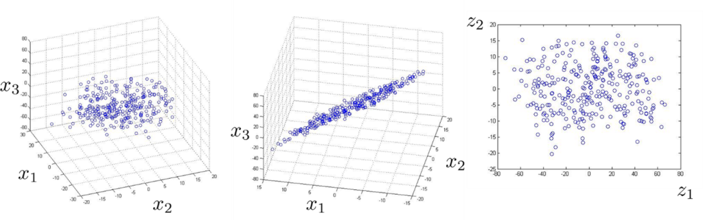
Figure. 5.1. Reducing the dimensionality of data from 3D to 2D

PCA can be used for many purposes, including data compression, feature extraction, and data visualization. In data compression, PCA is used to reduce the size of a dataset by reducing the number of features while preserving the maximum amount of information. In feature extraction, PCA is used to identify the most important features of a dataset, which can then be used for further analysis. In data visualization, PCA is used to plot high-dimensional data in two or three dimensions, making it easier to interpret and understand.
Overall, PCA is a powerful tool for dimensionality reduction that is widely used in many fields, including machine learning, data analysis, and data visualization. By finding the principal components of a dataset, PCA can help simplify complex data, making it easier to understand and work with. PCA achieves this by identifying the directions (principal components) along which the data varies the most.

Objectives of PCA

1. Reduce the dimensionality of data while retaining the most significant features.
2. Remove redundancy and correlations among features.
3. Facilitate visualization of high-dimensional data.
4. Preprocess data for computational efficiency in downstream machine learning models.

Let the dataset [latex]X[/latex] be a matrix of size [latex]n \times d[/latex], where [latex]n[/latex] is the number of observations (data points), and [latex]d[/latex] is the number of features (dimensions).

1. Standardization
   Before applying PCA, it is essential to standardize the dataset to ensure all features contribute equally. The standardized dataset [latex]Z[/latex] is calculated as:

   \begin{align} Z_{ij}=\frac{x_{ij}-\mu_j}{\sigma_j} \tag{5.1}\end{align}

   where [latex]x_{ij}[/latex] is the value of the [latex]j[/latex]-th feature for the [latex]i[/latex]-th observation, [latex]μ_j[/latex] is the mean of the [latex]j[/latex]-th feature, and [latex]σ_j[/latex] is its standard deviation.

2. Covariance Matrix
   PCA seeks to find directions in which the variance of the data is maximized. The covariance matrix of the standardized data  is computed as:

   \begin{align}C=\frac{1}{n-1}Z^TZ \tag{5.2} \end{align}

   Here, [latex]C[/latex] is a symmetric [latex]d\times d[/latex] matrix, where each element [latex]c_{jk}[/latex] represents the covariance between features [latex]j[/latex] and [latex]k[/latex].

3. Eigenvalues and Eigenvectors
   PCA identifies principal components by solving the eigenvalue problem for the covariance matrix [latex]C[/latex]:

   \begin{align}Cv_i=\lambda_i v_i, \tag{5.3} \end{align}

   where:

   – [latex]λ_i[/latex] is the [latex]i[/latex]-th eigenvalue, representing the variance along the corresponding eigenvector.
   – [latex]v_i[/latex] is the [latex]i[/latex]-th eigenvector, representing the direction of the [latex]i[/latex]-th principal component.

   The eigenvalues are sorted in descending order [latex](λ_1≥ λ_2≥⋯≥ λ_d).[/latex]

4. Principal Components
   The principal components are linear combinations of the original features, defined by:

   \begin{align}p_i = Zv_i,\tag{5.4} \end{align}

   where [latex]p_i[/latex] is the projection of the data onto the [latex]i[/latex]-th principal component

5. Dimensionality Reduction
   To reduce the dimensionality from [latex]d[/latex] to [latex]k (k < d)[/latex], the top [latex]k[/latex] eigenvectors corresponding to the largest eigenvalues are chosen. The reduced data matrix [latex]Z_k[/latex] is computed as: \begin{align}Z_k = ZV_k \tag{5.5} \end{align} where [latex]V_k=[v_1,v_2,…,v_k][/latex] is the matrix of the top [latex]k[/latex] eigenvectors.

 

Detailed Steps of PCA

1. Input Data
   Start with a dataset [latex]X[/latex] of size [latex]n\times d[/latex].
2. Standardize Data
   Center and scale the data to zero mean and unit variance to obtain [latex]Z[/latex].
3. Compute Covariance Matrix
   Derive the covariance matrix [latex]C[/latex] from [latex]Z[/latex].
4. Eigen Decomposition
   Compute the eigenvalues and eigenvectors of [latex]C[/latex]. Sort the eigenvalues and corresponding eigenvectors in descending order.
5. Select Principal Components
   Retain the eigenvectors corresponding to the top [latex]k[/latex] eigenvalues.
6. Project Data
   Transform the original dataset onto the lower-dimensional subspace spanned by the selected eigenvectors.

PCA Example

Suppose we have a 2D dataset:

[latex]X = \begin{bmatrix} 2.5 & 2.4 \\ 0.5 & 0.7 \\ 2.2 & 2.9 \\ 1.9 & 2.2 \\ 3.1 & 3.0 \\ 2.3 & 2.7 \\ 2.0 & 1.6 \\ 1.0 & 1.1 \\ 1.5 & 1.6 \\ 1.1 & 0.9 \end{bmatrix}[/latex]

1. Standardize Data
   Subtract the mean and divide by the standard deviation for each feature.
2. Covariance Matrix
   Compute the covariance matrix:

   \begin{align} C = \begin{bmatrix}
   0.6165 & 0.6150 \\
   0.6150 & 0.7165 \\
   \end{bmatrix}\end{align}

3. Eigenvalues and Eigenvectors
   Solve for eigenvalues: [latex]λ_1=1.2840[/latex] ,[latex]λ_2=0.0490[/latex].
   Eigenvectors: [latex]v_1=[0.6779,0.7352]^⊤[/latex], [latex]v_2=[-0.7352,0.6779]^⊤[/latex].
4. Select Top Principal Component
   Retain [latex]v_1[/latex] for dimensionality reduction.
5. Transform Data
   Project data onto the first principal component to obtain the reduced dataset.

Advantages of PCA

1. Reduces dimensionality, improving computational efficiency.
2. Removes multicollinearity by transforming correlated features into orthogonal components.
3. Enables data visualization in 2D or 3D.

Limitations of PCA

1. Assumes linear relationships between features.
2. Sensitive to scaling; requires careful standardization.
3. May lose interpretability of transformed features.

Applications of PCA

1. Data Visualization: Reduces high-dimensional data for 2D/3D visualization.
2. Preprocessing: Prepares data for machine learning algorithms.
3. Noise Reduction: Eliminates less informative components.
4. Image Compression: Reduces image dimensions while retaining critical details.

PCA remains an essential tool in the machine learning arsenal, enabling efficient and interpretable data analysis.

5.2. Linear Discriminant Analysis (LDA)

Linear Discriminant Analysis (LDA) is a supervised dimensionality reduction technique designed to maximize class separability while minimizing within-class variance. Unlike PCA, which is unsupervised, and variance focused, LDA explicitly incorporates class labels to identify optimal projection directions for classification tasks.

Objectives of LDA

1. Maximize Class Separability: Project data into a lower-dimensional space where classes are well-separated.
2. Minimize Within-Class Variance: Ensure samples from the same class cluster closely.
3. Dimensionality Reduction: Reduce the feature space while retaining essential class information.

Mathematical Foundation of LDA

Let [latex]X[/latex] be the dataset of size [latex]n\times d[/latex], where [latex]n[/latex] is the number of samples and [latex]d[/latex] is the number of features. Assume [latex]C[/latex] classes, labeled as [latex]C_1,C_2,…,C_C,[/latex] with [latex]n_c[/latex] samples in class [latex]C_c[/latex].

1. Mean Vectors:
   The mean vector for class [latex]C_c[/latex] is:

   \begin{align} \mu_c = \frac{1}{n_c} \sum_{x_i \in C_c} x_i \end{align}

   where [latex]x_i[/latex]is a sample from class [latex]C_c[/latex]. The global mean vector [latex]μ[/latex], representing the mean of all samples, is:

   \begin{align} \mu = \frac{1}{n} \sum_{i = 1} x_i \tag{5.6} \end{align}

2. Scatter Matrices:
   1. Within-Class Scatter Matrix [latex]S_W[/latex]: Measures the variance of samples within each class:
      \begin{align} S_W = \sum_{c=1}^C \sum_{x_i \in C_c} (x_i -\mu_c)(x_i-\mu_c)^T. \end{align}

      Alternatively, [latex]S_W[/latex] can be expressed as:

      \begin{align}S_W = \sum_{c=1}^C S_c \text{ },\tag{5.7} \end{align}

      where [latex]∑_{x_i∈C_c}(x_i-μ_c ) (x_i-μ_c )^T [/latex] is the scatter matrix for class [latex]C_c[/latex].

   2. Between-Class Scatter Matrix ([latex]S_B[/latex]): Measures the variance between class means:

      \begin{align}S_B = \sum_{c=1}^C n_c (\mu_c – \mu)(\mu_c – \mu)^T \tag{5.8} \end{align}

3. Optimization Objective:
   LDA seeks to maximize the separability of classes by maximizing the ratio of the determinant of the between-class scatter matrix to the within-class scatter matrix. This is equivalent to solving:

   \begin{align} w = \textit{argmax} \frac{W^TS_BW}{W^TS_WW}. \tag{5.9} \end{align}

   This optimization is performed using the generalized eigenvalue problem:

   \begin{align} S_B W = \lambda S_W W. \tag{5.10} \end{align}

   Here, λ represents the eigenvalues, and w is the corresponding eigenvector. The eigenvectors associated with the largest eigenvalues define the optimal projection directions.

4. Dimensionality Reduction:
   To reduce the dimensionality from [latex]d[/latex] to [latex]k (k ≤ min(C-1,d))[/latex], select the top [latex]k[/latex] eigenvectors corresponding to the largest eigenvalues. The reduced data [latex]Z[/latex] is given by:

   \begin{align} Z = XW ,\end{align}

   where [latex]W=[w_1,w_2,…,w_k][/latex] is the projection matrix.

LDA Algorithm

1.  Input: Dataset [latex]X[/latex] with class labels.
2. Compute Class Means: Calculate [latex]μ_c[/latex] for each class and the global mean [latex]μ[/latex].
3. Construct Scatter Matrices: Compute [latex]S_W[/latex] and [latex]S_B[/latex].
4. Solve Eigenvalue Problem: Perform eigen decomposition of [latex]S_{W}^{-1} S_B[/latex].
5. Select Top Components: Choose [latex]k[/latex] eigenvectors with the largest eigenvalues.
6. Project Data: Transform data using [latex]W[/latex].

Example of LDA

Suppose a 2-class dataset:

[latex]X = \begin{bmatrix} 2.5 & 2.4 \\ 0.5 & 0.7 \\ 2.2 & 2.9 \\ 1.9 & 2.2 \\ 3.1 & 3.0 \\ 2.3 & 2.7 \\ 2.0 & 1.6 \\ 1.0 & 1.1 \\ 1.5 & 1.6 \\ 1.1 & 0.9 \end{bmatrix}[/latex]

with labels [latex]y=[1,1,1,1,1,2,2,2,2,2][/latex].

1. Compute class mean vectors [latex]μ_1[/latex], [latex]μ_2[/latex], and global mean [latex]μ[/latex].
2. Construct [latex]S_W[/latex] and [latex]S_B[/latex].
3. Solve the eigenvalue problem and project the data.

Advantages of LDA

1. Incorporates class information for dimensionality reduction.
2. Finds optimal projection directions for class separation.
3. Efficient for classification tasks.

Limitations of LDA

1. Assumes linear separability of classes.
2. Requires normally distributed features within each class.
3. Sensitive to outliers.

Applications of LDA

1. Classification: Preprocessing for machine learning models.
2. Face Recognition: Reducing dimensionality in image datasets.
3. Medical Imaging: Distinguishing disease states.
4. Finance: Pattern recognition in market data.

By integrating LDA into workflows, students can effectively address classification challenges where dimensionality reduction and class separability are critical.

5.3. Isometrically Mapping Background

MDS seeks to identify underlying dimensions that may help to describe differences among HD features, which is the base for isometric mapping. To deal with nonlinear complicated data, there are solutions to be followed. One way is to use kernel methods to project data to an HD space where we can linearly group data. Another approach is to use nonlinear methods to unfold the nonlinearity in the data. Isomap uses geodesic distance to unfold the HD manifolds to a simpler one and makes them easier to project to LD space.

Our data points can be shown as a combination of multiple vectorized data points, [latex]X=[x_1,x_2,…,x_n ]∈\mathbb{R}^{d\times n}[/latex], where [latex]\{x_i∈R^d\}_{i=1}^n[/latex]. We assume that there is a finite data point drawn from our [latex]X[/latex]. We can build a geometric graph [latex]G=(V;E)[/latex] that has our data points as vertices and connects vertices that are close to each other. We construct a k-nearest neighbor graph for the [latex]x_i[/latex] connected to [latex]x_j[/latex] correspondingly and for [latex]x_j[/latex] to [latex]x_i[/latex], show them by [latex]γ(x_i )[/latex] and [latex]γ(x_j ) (γ(x_i ),γ(x_j )∈ M)[/latex]. [latex]γ(.)[/latex] represents a vector point on the manifold. The length of the path is defined by summing the edge weights along the path on the manifold. The shortest path ([latex]\mathcal{S}\mathcal{P}[/latex]) distance [latex]D_{\mathcal{S}\mathcal{P}}[/latex][latex](γ(x_i ),γ(x_j ))[/latex] between two vertices [latex]γ(x_i ),γ(x_j )∈V[/latex] and defines based on the length of the [latex]\mathcal{S}\mathcal{P}[/latex] connecting them.
[latex]g(.)[/latex] is a positive continuous scalar function for [latex]X[/latex] in the given path [latex]γ(.)[/latex] connecting [latex]x_i[/latex] and [latex]x_j[/latex], which is parameterized by g-length of the path as
\begin{align} D_{g,y} = \int_y g(y(t))|y'(t)|dt \tag{5.11 }\end{align}

Where [latex]γ' (.)[/latex] defines a small element on the manifold, also known as the line integral along the path [latex]γ(.)[/latex] with respect to [latex]g(.)[/latex]. [latex]D_{g,γ}[/latex] denotes distance on the manifold through the shortest path. The g-geodesic path connecting [latex]x_i[/latex] and [latex]x_j[/latex] is the path with minimized g-length. The shortest path is used for the Isomap algorithm to find the path on the HD manifold for connecting two points.

We assume that the LD embedding of the training data with the respect to the vectorized data points of the observation can be shown as [latex]Y=[y_1, y_2,…,y_n ]∈\mathbb{R}^{p\times n}[/latex], where [latex]\{y_i∈R^p\}_{i=1}^n[/latex], where [latex]p \leq d[/latex], desirably and usually [latex]p≪d[/latex]. The MDS method aims to project similar points of the data close to each other and dissimilar points as far as possible. This is followed by the equation below:

\begin{align}\underset{Y}{min}||D_{g,y}(X) – D_{g,y}(Y)||_F^2 \tag{5.12 }\end{align}

where [latex]D_{g,γ}[/latex] is the shortest path distance from equation (5.11). [latex]D_{g,γ} (X)[/latex] and [latex]D_{g,γ} (Y)[/latex] are any pairwise distances of the data in HD space and in the subspace and can be written by similarity [latex]X^T X[/latex] and [latex]Y^T Y[/latex] in the projected

space. In MDS, the solution for this problem is [latex]Y=Δ^{1/2} V^T[/latex], where [latex]V^T[/latex] and [latex]Δ[/latex] are the eigenvector and eigenvalue matrices of the input data, [latex]X[/latex]. This is equivalent to the PCA method. If we use a generalized kernel with the respect to the kernel distance matrix [latex]D[/latex] as:

\begin{align} -\frac{1}{2} HDI \tag{5.13 } \end{align}

with the centering matrix of [latex]H,H=I-\frac{1}{n} 11^T[/latex]. In generalized MDS embedding we use eigen decomposition of [latex]K[/latex]. MDS applies Euclidean distance for finding the distance of the data vectors and their similarity measurement. In HD space and curved manifolds, Euclidean distance might not solve the distance between the points on the manifold. In other words, intrinsic and extrinsic distances between two points in the curved manifold of data in the space might not be the same. Isomap solved this problem by using the geodesic distance between the points on the HD manifold. Isomap algorithm comprises two main steps:

1.  Creating a k-nearest-neighbor graph in HD space of the points on the manifold, and then calculating the geodesic distance between each pair of points applying shortest-path distance.
2. Employing MDS and making the distance matrix to locate the points in the embedded lower dimensional space.

Isomap follows the Cayton assumptions to retrieve the manifold parametrization:

• An isometric embedding of the manifold in [latex]\mathbb{R}^p[/latex] exists.
• The manifold in [latex]\mathbb{R}^d[/latex] is convex as well as its parameter space. In other words, there is no hole in the manifold. Also, geodesic distance between any two points in the parameter space remains entirely in the parameter space.
• Everywhere on the manifold points are sufficiently sampled.
• The compactness of the manifold topologically.

Increasing the distance between the paired points mitigates the similarity of these two distances and the accuracy of such an approximation, which ultimately leads to the original MDS problem.

5.4. PR – Constraint Isometric Mapping
The Isomap algorithm creates a k-nearest neighbor graph and uses the shortest path algorithm to estimate the geodesic distances between points. After finding geodesic distances between points, it searches for geodesic distances equivalent to Euclidean distances. Due to isometrically embedded manifold conditions, some points satisfy these conditions along with translation and rotation, i.e., MDS is a classic example of finding these points.

This study focuses on the Isomap algorithm for nonlinear manifold learning, which aims to maintain the pairwise geodesic distances between data points. To calculate the geodesic distance in the shortest path between two data points, we suppose that the data points belong to [latex]d[/latex]-dimensional manifold embedded in [latex]\mathbb{R}^d[/latex] ambient space. The crucial assumption for the Isomap method is the presence of an isometric chart, which pair points such as [latex]x_i,x_j[/latex] lie on the HD manifold. [latex]D_{g,γ} (x_i,x_j )[/latex] denotes the geodesic distance of the pairwise points [latex]γ:M→ \mathbb{R}^d[/latex] such that:

\begin{align} D_{g,γ} (x_i,x_j ) ∝||γ(x_i )-γ(x_j )||_2 \tag{5.14 } \end{align}

where [latex]x_i[/latex] and [latex]x_j[/latex] are near each other on the manifold. Geodesic distance of [latex]γ(x_i )[/latex] and [latex]γ(x_j ), γ(x_i ),γ(x_j )∈ M[/latex] defines along the manifold surface, [latex]M[/latex], and is denoted by [latex]D_(g,γ) (x_i,x_j )[/latex].

By building a neighborhood graph where each point is connected exclusively to its k nearest neighbors, Isomap first calculates an estimate of the geodesic distances between every pair of data points located on the manifold [latex]M[/latex]; the edge weights are equivalent to the corresponding pairwise distances. The Euclidean distance serves as an estimate for the geodesic distance for adjacent pairs of data points. This assumption allows finding an approximation of [latex]D_(g,γ) (x_i,x_j )[/latex] applying many small Euclidean distances, i.e.,
\begin{align}
D_{g,γ} (x_i,x_j )≈||γ(x_i )-γ(x_j )||_2 \text{ }\text{   for   } \text{ } γ(x_j )∈N_k (γ(x_j )), \tag{5.15 }\end{align}

where [latex]N_k (γ(x_j ))[/latex] denotes the collection of the point [latex]γ(x_i )∈ M[/latex] for k closest neighbors on the manifold surface, M. The geodesic distance is calculated for non-neighboring points as the shortest path length along the neighborhood graph, which can be discovered using Dijkstra’s algorithm. The generated geodesic distance matrix is then subjected to MDS to identify a group of LD points that most closely match such distances.

Forming a k-nearest neighbor graph for the data points might create inconsistency between geodesic and Euclidean distances in opposition to the aforementioned condition. Particularly, if the third Cayton assumption does not or is weakly satisfied. It indirectly implies that points in the HD manifold should be uniformly distributed. If otherwise, for large k in the k-nearest neighbor graph there will be cases that create a discrepancy in an approximation of the geodesic and Euclidean distances. This will cause a difference between intrinsic and extrinsic distances on the manifold.

Figure 5.2. Geometric interpretation of the shortest path and PR-Isomap under [latex]N_{k,h} (γ(x_k ))[/latex], Parzen–Rosenblatt window constraint on k-nearest neighbor windows on HD manifold (a) and in the LD space after PR-Isomap projection (b). [latex]d_{Euc} x_a,x_b[/latex] and [latex]D_{g,γ} (x_a,x_b )[/latex] are Euclidian and geodesic distances between [latex]x_a[/latex] and [latex]x_b[/latex].

Here, we tackle this problem using the Parzen–Rosenblatt window constraint on the k-nearest neighbor for a weak-uniformly distributed manifold which enforces the accuracy of distance approximation in Isomap algorithm.

Definition 1: Parzen–Rosenblatt (PR) window is defined as

\begin{align} p_h(x)= \frac{1}{k}\sum_{i=1}^k \frac{1}{h^2} Φ( \frac{x_i – x}{h}) \tag{5.16 }\end{align}

let [latex]k[/latex] as number of neighbors centered in the vector, [latex]x[/latex], [latex]p_h (x)[/latex] denotes the probability density of [latex]x[/latex], while [latex]h[/latex] is the dimension of the window that satisfies the approximation of geodesic and Euclidean distances, and [latex]Φ[/latex] represents the window function, here it can be a rectangle function, uniform distribution, like a window function with the size [latex]h[/latex]. This function is also called the density estimation function.

Additionally, PR-Isomap alters the graph weights of a portion of each point’s k-nearest neighbors with respect to the pairwise distance of the points on the manifold surface, [latex]M[/latex], that meet the requirements for the PR window. The set of points in a PR-based point around each point [latex]γ(x_i ), γ(x_i )∈ M[/latex] are considered for projection as neighboring elements. Suppose that the point [latex]γ(x_j )[/latex], where [latex]γ(x_i )∈ N_{k,h} (γ(x_j ))[/latex] is the closest matching point that can be used for measuring the distance [latex]D_{g,γ} (x_i,x_j )[/latex], i.e.,

\begin{align} \underset{γ(x_k )∈ N_{k,h} (γ(x_k ))}{min} D_{g,y}(x_i,x_j) \tag{5.17 } \end{align}

PR-based isometric mapping uses a subset of k-nearest neighbor with a distance less than h on the surface of the manifold, M, which is represented by uniform neighbors [latex](\mathcal{U}\mathcal{N}(x_i)[/latex]), i.e.,

\begin{align} \mathcal{U}\mathcal{N}(x_i)=\begin{Bmatrix}
γ(x_i )∈M,\text{ }\text{ }\text{ }\text{ }\text{ }\text{ }\text{ }γ(x_i )∈ N_{k,h} (γ(x_i )), \\
D_{g,γ} (x_i,x_j ) \leq \underset{γ(x_k )∈ N_{k,h} (γ(x_k ))}{min}D_{g,γ} (x_i,x_k )
\end{Bmatrix} \tag{5.18 } \end{align}

In other words, [latex]\mathcal{U}\mathcal{N}(x_i )[/latex] is a subset of the nearest neighbor graph, which falls into the PR radius, containing points on the manifold [latex]M[/latex] which are closer to the targeted point out of the entire trivial match. [latex]\mathcal{U}\mathcal{N}[/latex] points are employed to detect data points on the local neighborhood of every point [latex]γ(x_i )[/latex] with a higher expectation to be analogous to [latex]γ(x_i )[/latex].

Using MDS generalized optimization:

\begin{align} \underset{Y}{min}||D_{g,γ} (X)-D_{g,γ} (Y)||_F^2 \tag{5.19 } \end{align}

\begin{align} \text{subject to } D_{g,γ} (x_i,x_j )≤ h \end{align}

where [latex]D_{g,γ}[/latex] (X) redefines as any pairwise distances on the surface of the HD manifold, [latex]M[/latex], while the [latex]\mathcal{S}\mathcal{P}[/latex] distance using an unweighted PR-based k-nearest neighbor graph, [latex]p_h[/latex]. Figure 5.2 presents the geometrical interpretation of the shortest path and PR-Isomap under [latex]N_{k,h} (γ(x_k ))[/latex], where PR-window constraints the k-nearest neighbor path.

 

 

 

References

Yousefi, B., Khansari, M., Trask, R., Tallon, P., Carino, C., Afrasiyabi, A., … & Hershman, M. (2024). Density-based Isometric Mapping. arXiv preprint arXiv:2403.02531.

Yousefi, M. Khansari, R. Trask, P. Tallon, C. Carino, A. Afrasiyabi, V. Kundra, L. Ma, L. Ren, K. Farahani, M. Hershman (2024). Measuring Subtle HD Data Representation and Multimodal Imaging Phenotype Embedding for Precision Medicine. IEEE Transactions on Instrumentation and Measurement, TIM-24-01821-in press.